Mean Squared Error (MSE) as a Loss Function
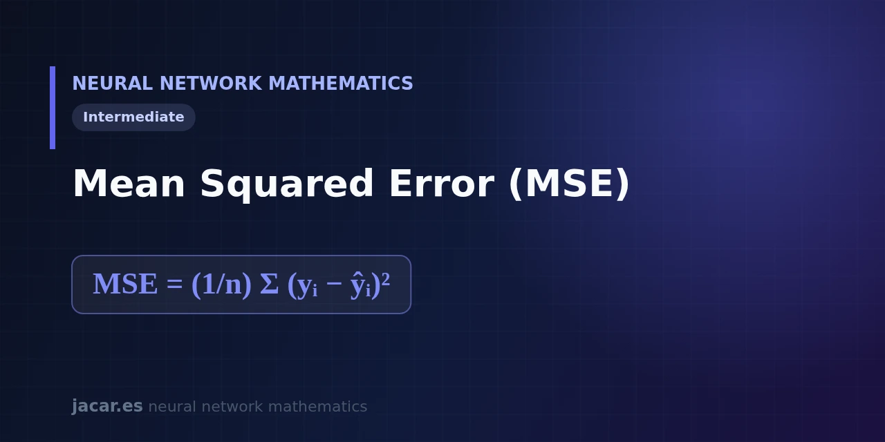
Table of contents
Mean squared error (MSE) is the loss function that measures, on average, how far each prediction sits from the true value by squaring that gap. It is the default choice for regression problems and the first error criterion almost everyone learns. Its form is short, but the choice to square the difference has deep consequences: it makes the function differentiable everywhere and turns a large mistake into a disproportionate penalty. The same explanation is available in Spanish.
Key takeaways
- The mean squared error averages the square of the gap between each true value $y_i$ and its prediction $\hat{y}_i$, with the formula $\mathrm{MSE} = \frac{1}{n}\sum(y_i-\hat{y}_i)^2$.
- Its derivative with respect to the prediction is proportional to the error itself, $\frac{2}{n}(\hat{y}_i-y_i)$, which gives gradient descent a clean signal.
- By squaring, an error of 10 weighs 100 times more than an error of 1: that is why MSE chases big mistakes so hard.
- The same property makes it sensitive to outliers, since a single extreme point can dominate the loss.
- It is the reference loss for regression, whereas classification defaults to cross-entropy.
What is the MSE?
MSE is a loss function: a single number that summarises how badly a model is doing over a dataset. The lower the better; an MSE of 0 means the predictions match reality exactly.
The idea is as old as the method of least squares that Gauss and Legendre popularised in the early nineteenth century. As statistics historian Stephen Stigler puts it, «the method of least squares is the automobile of modern statistical analysis». In machine learning that same criterion reappears as the loss we minimise when training a regression model, whether a straight line or a neural network with millions of parameters.
The name says it all: it is the mean of the squared error. It is computed over $n$ examples, and each one contributes the square of its individual deviation.
Formula and its derivative
The formal definition is:
$$\mathrm{MSE} = \frac{1}{n}\sum_{i=1}^{n}(y_i-\hat{y}_i)^2$$
where $y_i$ is the true value of example $i$, $\hat{y}_i$ is the model’s prediction, and $n$ is the number of examples. The difference $y_i-\hat{y}_i$ is called the residual.
What makes MSE useful for training is its derivative. For a single prediction, the derivative of $(y_i-\hat{y}_i)^2$ with respect to $\hat{y}_i$ is $-2(y_i-\hat{y}_i)$. Averaging over the $n$ examples, the gradient becomes:
$$\frac{\partial \mathrm{MSE}}{\partial \hat{y}_i} = \frac{2}{n}(\hat{y}_i-y_i)$$
Show the derivation
Apply the chain rule to the term $(y_i-\hat{y}_i)^2$. The power rule leaves $2(y_i-\hat{y}_i)$, and the inner derivative of $(y_i-\hat{y}_i)$ with respect to $\hat{y}_i$ is $-1$; multiplying gives $-2(y_i-\hat{y}_i)$. Since the MSE averages those terms, the $\frac{1}{n}$ factor is kept and, reordering the sign, we obtain $\frac{\partial \mathrm{MSE}}{\partial \hat{y}_i} = \frac{2}{n}(\hat{y}_i-y_i)$.
The key detail is that the gradient is proportional to the error: the farther the prediction, the larger the corrective push, and when the prediction is right, the gradient vanishes. That smoothness is what pairs so well with gradient descent, the machinery covered in the mathematics of neural networks roadmap. For convenience, the loss is also defined as $\frac{1}{2n}\sum(y_i-\hat{y}_i)^2$, so the factor of 2 in the derivative cancels and leaves $\frac{1}{n}(\hat{y}_i-y_i)$.
Why it punishes large errors
Squaring is not a neutral choice. An error of 2 units contributes 4 to the sum, but an error of 4 units contributes 16: doubling the error quadruples the penalty. And an error of 10 weighs 100 times more than an error of 1.
The practical consequence is that MSE penalises one huge mistake more than the same amount of error spread across small ones. A model optimised with MSE tunes its weights, above all, to remove the largest errors, even if that slightly worsens already-good predictions. That is exactly what we want when a big error tends to be more costly than the sum of small ones. The square root of the MSE, the RMSE, undoes the square and returns the error to its original units, which makes it easier to read.
Sensitivity to outliers
The flip side of that virtue is a well-known flaw: MSE is sensitive to outliers. Because a single large residual is squared, one extreme point (a measurement error, a genuine anomaly) can dominate the loss and drag the whole fit towards it.
When that sensitivity gets in the way, the usual alternative is the mean absolute error (MAE), which uses the absolute value instead of the square and treats all errors proportionally. There are intermediate options too, such as the Huber loss, which behaves like MSE near zero and like MAE far from it. Choosing between MSE and MAE depends on whether the outliers in your data are signal you want to capture or noise you want to ignore.
Before settling on a loss, inspect your data. A single outlier can multiply the MSE by tens and drag the whole fit towards it. Decide deliberately whether that extreme point is signal you want to capture or noise you want to clean out.
Numerical example
Suppose four true values $[10, 12, 14, 16]$ and these predictions $[11, 11, 15, 16]$. The residuals are $-1, 1, -1, 0$; their squares, $1, 1, 1, 0$. The sum is 3 and, with $n = 4$, the MSE is $3/4 = 0.75$. The RMSE is $\sqrt{0.75} \approx 0.87$, meaning the model is off by less than one unit on average.
Now we add an outlier: we change the last prediction from 16 to 6, so its residual becomes 10 and its square, 100. The new sum is $1+1+1+100 = 103$ and the MSE jumps to $103/4 = 25.75$. A single data point has multiplied the loss by 34, from $0.75$ to $25.75$, while the other three examples are still predicted just as well. This contrast shows, in numbers, why MSE chases big mistakes and why an outlier can skew training.
Frequently asked questions
What is the difference between MSE and RMSE?
RMSE is the square root of the MSE. They rank models the same way (whatever minimises one minimises the other), but RMSE is in the same units as the target variable. That makes it directly interpretable: an RMSE of $0.87$ means a typical error of $0.87$ units.
When should I use MSE instead of MAE?
Use MSE when large errors are especially costly and you want the model to prioritise them, or when you need a loss that is differentiable everywhere. Prefer MAE when your data has outliers you regard as noise and you do not want them to dominate the fit.
Why is MSE not used for classification?
Because in classification the output is a probability and the target is a label; there cross-entropy gives more useful gradients and more stable optimisation. MSE is reserved for regression, where a continuous value is predicted.
Conclusion
Mean squared error is the gateway to loss functions: a short formula with a definite behaviour. Squaring gives it a smooth derivative, ideal for gradient descent, and a healthy obsession with large errors, at the cost of strong sensitivity to outliers. Understanding that trade-off is the first step to choosing the right loss for each problem. The next is comparing MSE with MAE and cross-entropy within the mathematics of neural networks roadmap.