Batch Normalization
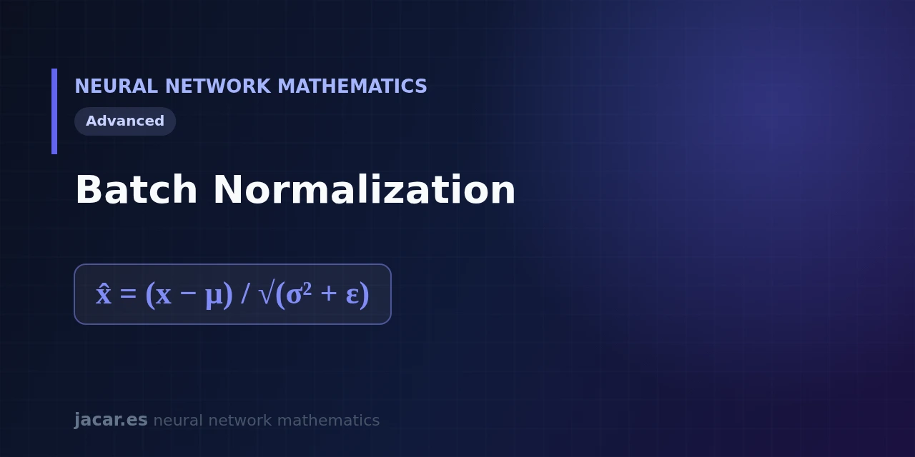
Table of contents
- Key takeaways
- What is batch normalization?
- The formula (normalise, scale and shift)
- Gamma and beta, the learnable parameters
- Why it speeds up training
- Training versus inference
- Frequently asked questions
- How does it differ from layer normalization?
- Can I use small batches?
- Is the bias in the previous layer still needed?
- Conclusion
- Sources
Batch normalization rescales each layer’s activations so they have zero mean and unit variance within every mini-batch, letting training move faster and with fewer stumbles. It is one of the tools that made deep networks trainable in practice. This guide covers what it does, its formula, what its two learnable parameters are for and why it behaves differently during training and prediction. The same explanation is available in Spanish.
Key takeaways
- Batch normalization normalises a layer’s activations by subtracting the mini-batch mean and dividing by its standard deviation, then rescales them with two learnable parameters.
- Sergey Ioffe and Christian Szegedy proposed it in 2015 to fight what they called internal covariate shift.
- Its gamma (scale) and beta (shift) parameters give the network back the ability to represent any range of values, even to undo the normalization if that is optimal.
- It allows higher learning rates and makes training much less sensitive to weight initialisation.
- During training it uses mini-batch statistics; at inference it uses means and variances accumulated during training.
What is batch normalization?
In a deep network, the distribution of each layer’s inputs shifts constantly as the weights of earlier layers are updated. That drift forces you to lower the learning rate and slows convergence. Batch normalization tackles it by normalising each layer’s input separately, not once at the start but at every training step.
The idea was introduced by Sergey Ioffe and Christian Szegedy in the 2015 paper «Batch Normalization: Accelerating Deep Network Training by Reducing Internal Covariate Shift»[1]. In their experiments with the Inception network on ImageNet, they reached the baseline accuracy with 14 times fewer training steps. An ensemble with batch normalization pushed the top-5 error down to 4.9%, beating the estimated human accuracy on that task.
As the authors themselves put it, «Batch Normalization allows us to use much higher learning rates and be less careful about initialization, and in some cases eliminates the need for Dropout».
The formula (normalise, scale and shift)
Inside a mini-batch, each activation $x$ is normalized in two steps: first it is standardised using the batch’s own mean and variance, then it is rescaled with two learnable parameters.
$$\hat{x} = \frac{x-\mu}{\sqrt{\sigma^2+\varepsilon}}, \qquad y = \gamma\hat{x}+\beta$$
In PyTorch both steps are wrapped in a single layer:
import torch.nn as nn

bn = nn.BatchNorm1d(256, eps=1e-5, momentum=0.1)  # normalises 256 channels
y = bn(x)  # y = gamma * x_norm + beta
In the standardisation, $\mu$ is the mini-batch mean, $\sigma^2$ its variance and $\varepsilon$ a small constant (0.00001 by default in PyTorch) that avoids dividing by zero. The rescale $y = \gamma\hat{x}+\beta$ is the second step. This operation goes between the weighted sum $z = \mathbf{W}x+b$ and the activation function $a = f(z)$, though its exact position has variants. You can review the weighted sum in the mathematics of neural networks roadmap.
The constant $\varepsilon$ only comes into play when the batch variance is tiny. It prevents division by zero without altering the result in practice, because its default value of 0.00001 is far smaller than any real variance.
Gamma and beta, the learnable parameters
If we kept only the standardisation, we would force every layer to have zero mean and unit variance, which would limit what the network can represent. That is why two parameters are added that the network learns just like the weights: $\gamma$ (gamma) scales the result and $\beta$ (beta) shifts it.
The key point is that these two parameters let the network undo the normalization when it helps. If the optimal values were $\gamma = \sqrt{\sigma^2+\varepsilon}$ and $\beta = \mu$, the layer would recover exactly the original activation. In other words, the network loses no expressive power: it only gains an easier path to the solution. Each channel or feature has its own gamma and beta pair, so a layer with 256 channels adds 512 learnable parameters, a tiny amount next to the weights.
Show the derivation
Substituting those optimal values into the rescale: $y = \gamma\hat{x}+\beta = \sqrt{\sigma^2+\varepsilon}\cdot\dfrac{x-\mu}{\sqrt{\sigma^2+\varepsilon}}+\mu = (x-\mu)+\mu = x$. The layer reconstructs the original input, so normalization never costs the network any expressive power.
Why it speeds up training
Why it works is still debated. Ioffe and Szegedy attributed it to reducing internal covariate shift, the change in the distribution of activations layer by layer. In 2018, an MIT team questioned that in «How Does Batch Normalization Help Optimization?»[2]: they showed the main effect is smoothing the loss surface, making gradients more predictable and stable, which allows larger steps without training blowing up.
Whatever the explanation, the practical effects are clear: it converges in fewer epochs, tolerates higher learning rates and reduces dependence on careful initialisation. It also adds a mild regularising effect, because the mini-batch noise acts as a perturbation. That effect connects to problems such as the exploding gradient, which normalization helps to contain.
Training versus inference
Here is the detail that trips people up most. During training, the layer normalises with the mean and variance of the current mini-batch, which change at every step. But at inference the model may process a single example, and normalising against a batch of size one would make no sense.
The solution is to accumulate during training a running mean and variance of the whole population. PyTorch updates them with a momentum factor of 0.1 by default and stores them as model statistics. When you call model.eval(), the layer stops using the batch and applies those fixed statistics, so the output is deterministic and does not depend on which other examples it travels with.
Forgetting that mode switch is a common source of erratic results in production. The behaviour is documented in the PyTorch reference[3].
Frequently asked questions
How does it differ from layer normalization?
Batch normalization computes the mean and variance over the batch dimension, for each channel. Layer normalization computes them over the features of a single example, so it does not depend on the batch size. That is why transformers, with variable-length sequences, tend to prefer layer normalization.
Can I use small batches?
With batches of 2 or 4 examples the mean and variance are estimated with a lot of noise and the technique loses effectiveness. In those cases people turn to alternatives such as group normalization, designed for small batch sizes in computer vision.
Is the bias in the previous layer still needed?
No. Because normalization subtracts the mean, any bias $b$ in the previous layer cancels out. That is why a layer followed by batch normalization drops its bias: it is a parameter that would add nothing.
Conclusion
Batch normalization was one of the advances that made deep networks trainable: it normalises each layer with mini-batch statistics, rescales it with gamma and beta, and switches to accumulated statistics at inference. Although the exact reason is still argued over, its practical effect of stabilising and speeding up training is beyond doubt. The natural next step is to understand how it relates to weight initialisation and to the vanishing gradient.
Sources: [1] Batch Normalization (Ioffe and Szegedy, 2015)[1], [2] Batch normalization (Wikipedia)[4], [3] torch.nn.BatchNorm1d (PyTorch documentation)[3].