Weight Initialization: Xavier/Glorot and He
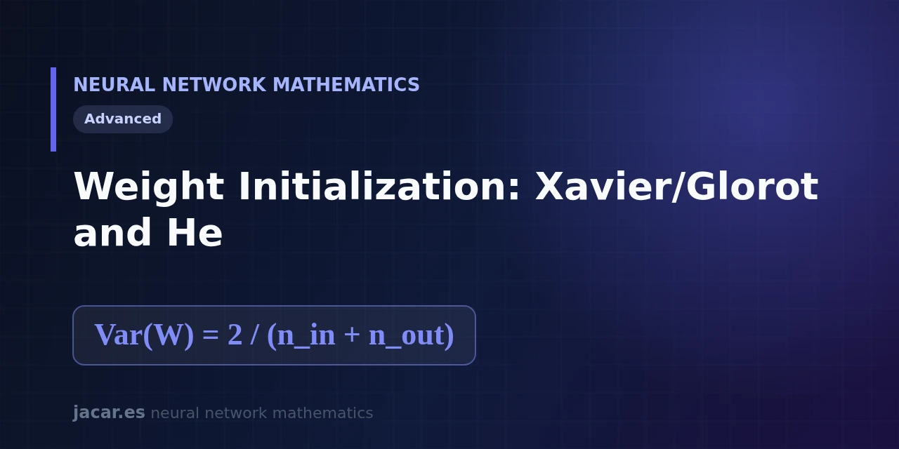
Table of contents
- Key takeaways
- Why initialization matters
- The activation variance problem
- Xavier/Glorot initialization
- He (Kaiming) initialization for ReLU
- Practical rules
- Frequently asked questions
- Why can't I initialize all weights to zero?
- When do I use Xavier and when do I use He?
- Does initialization still matter with batch normalization?
- Conclusion
- Sources
Weight initialization decides which numbers a network starts from before it sees a single data point, and that choice determines whether training moves forward or stalls. When the initial weights have the wrong scale, the signal flowing through the layers either fades to nothing or grows out of control. Xavier/Glorot and He are two simple recipes that set the right variance for each activation type.
This guide explains where they come from and when to use each one. The same explanation is available in Spanish.
Key takeaways
- Weight initialization means choosing the initial values of the matrix
Wbefore training; the goal is to keep the variance of the activations stable layer by layer. - Setting every weight to zero breaks learning: all neurons in a layer would compute the same thing and receive the same gradient.
- Xavier/Glorot initialization, published in 2010, uses $\operatorname{Var}(W) = \tfrac{2}{n{\text{in}} + n{\text{out}}}$ and is meant for symmetric activations such as sigmoid and the hyperbolic tangent.
- He initialization, from 2015, doubles that value to $\operatorname{Var}(W) = \tfrac{2}{n_{\text{in}}}$ to compensate for ReLU zeroing half of the activations.
- The practical rule is direct: ReLU and its variants call for He; sigmoid and tanh call for Xavier; the biases
bare set to 0.
Why initialization matters
A neural network is a chain of layers, and each one computes $z = Wx + b$ and then applies an activation $a = f(z)$. If the weights start too small, each layer shrinks the magnitude of the signal and, after 10 or 20 layers, the activations are practically zero. If they start too large, the opposite happens and the values explode. At either extreme, the gradient flowing backward during backpropagation becomes useless, an effect we cover in depth in the vanishing gradient problem.
There is one case worth ruling out immediately: initializing every weight to the same value, say 0. If two neurons in a layer start out identical and receive the same input, they produce the same output and the same gradient, so they update in lockstep forever. The network never breaks that symmetry and wastes neurons. That is why weights are drawn at random from a distribution with mean 0 and a carefully chosen variance.
The activation variance problem
The key is to control how the variance changes from one layer to the next. Assume independent inputs and weights, each with mean 0. For the weighted sum $z = Wx$, the variance of each output is $\operatorname{Var}(z) = n{\text{in}} \cdot \operatorname{Var}(W) \cdot \operatorname{Var}(x)$, where $n{\text{in}}$ is the number of inputs to the neuron (the fan-in).
If we want the output variance to match the input variance, we need $n{\text{in}} \cdot \operatorname{Var}(W) = 1$, that is $\operatorname{Var}(W) = \tfrac{1}{n{\text{in}}}$. This is LeCun’s intuition from 1998. The catch is that a network also propagates gradients backward, and there the number of outputs $n{\text{out}}$ (the fan-out) rules: for the gradient not to shrink you need $n{\text{out}} \cdot \operatorname{Var}(W) = 1$. Since $n{\text{in}}$ and $n{\text{out}}$ rarely match, a compromise is needed.
Show the derivation
For the weighted sum $z = \sum_{i=1}^{n_{\text{in}}} W_i x_i$ with independent weights and inputs of mean 0, the variance of a sum of independent products is the sum of the variances, so $\operatorname{Var}(z) = n_{\text{in}} \cdot \operatorname{Var}(W) \cdot \operatorname{Var}(x)$. To keep the variance unchanged across the layer we impose $\operatorname{Var}(z) = \operatorname{Var}(x)$, which requires $n_{\text{in}} \cdot \operatorname{Var}(W) = 1$ and therefore $\operatorname{Var}(W) = \tfrac{1}{n_{\text{in}}}$. Xavier averages that condition with the backward-pass one, $n_{\text{out}} \cdot \operatorname{Var}(W) = 1$, to reach $\tfrac{2}{n_{\text{in}} + n_{\text{out}}}$.
Xavier/Glorot initialization
Xavier Glorot and Yoshua Bengio proposed in 2010 to average the two conditions above. Instead of satisfying only the forward pass or only the backward pass, they take the mean of $n{\text{in}}$ and $n{\text{out}}$ and arrive at the formula that titles this guide:
$$\operatorname{Var}(W) = \frac{2}{n{\text{in}} + n{\text{out}}}$$
In practice two equivalent variants are used. The normal one draws weights from a Gaussian with that variance. The uniform one spreads them over the interval $[-r, r]$ with $r = \sqrt{6/(n{\text{in}} + n{\text{out}})}$, whose value yields exactly the same variance.
Glorot and Bengio showed that, with this scale, the activations of a network with the hyperbolic tangent keep a healthy variance across dozens of layers. The classic initialization of the time, by contrast, made them collapse. It is the default for activations centred on zero such as sigmoid or tanh, and it remains the one libraries like Keras pick for their dense layers.
The normal and uniform variants of Xavier produce the same variance: the uniform one only changes the shape of the distribution, not its scale. That is why you can swap one for the other without retuning the rest of the network.
He (Kaiming) initialization for ReLU
ReLU changed the rules. By discarding all negative values, $f(z) = \max(0, z)$ lets through on average only half of the activations, which halves the variance at each layer. Kaiming He and his co-authors analysed this in 2015 and corrected the factor: since ReLU keeps half, you compensate by doubling the variance of the weights.
$$\operatorname{Var}(W) = \frac{2}{n_{\text{in}}}$$
That is He initialization, also called Kaiming. With it, He and his team managed to train from scratch a 30-layer convolutional network on ImageNet, something that would not converge with Xavier. As the authors of the 2015 paper put it, their method «enables us to train extremely deep rectified models directly from scratch».
For leaky ReLU variants the formula adds a small adjustment based on the negative slope, but the factor of 2 remains the reference. It is PyTorch’s default for linear and convolutional layers.
Practical rules
With two recipes and a handful of caveats, almost any network ends up well initialized:
- ReLU or a variant (ELU, GELU, Leaky ReLU): use He with $\operatorname{Var}(W) = \tfrac{2}{n_{\text{in}}}$.
- Sigmoid or tanh: use Xavier/Glorot with $\operatorname{Var}(W) = \tfrac{2}{n{\text{in}} + n{\text{out}}}$.
- Biases: initialize them to 0; they do not suffer the symmetry problem because the weights are already different.
- Self-normalizing network with SELU: use the LeCun variant with $\operatorname{Var}(W) = \tfrac{1}{n_{\text{in}}}$.
- When in doubt: start from He, measure the variance of the activations in the first layers and adjust.
In code, picking the right recipe takes one line:
import torch.nn as nn

layer = nn.Linear(256, 128)
nn.init.kaiming_normal_(layer.weight, mode="fan_in", nonlinearity="relu")
nn.init.zeros_(layer.bias)
These recipes coexist with later techniques, such as batch normalization, that reduce sensitivity to initialization but do not replace it. To place this topic within the full route, see the mathematics behind neural networks roadmap.
Frequently asked questions
Why can’t I initialize all weights to zero?
Because the neurons in a layer would be identical: with the same input they compute the same output and receive the same gradient, so they update in the same way at every step. The network never breaks that symmetry and every neuron in a layer ends up computing the same thing. A random draw with mean 0 avoids the problem.
When do I use Xavier and when do I use He?
It depends on the activation. If the layer uses a symmetric function such as sigmoid or the hyperbolic tangent, Xavier/Glorot spreads the variance well with $\tfrac{2}{n{\text{in}} + n{\text{out}}}$. If it uses ReLU or one of its variants, He doubles it to $\tfrac{2}{n_{\text{in}}}$ to compensate for the half of the activations that ReLU sets to zero.
Does initialization still matter with batch normalization?
Yes, though less. Batch normalization rescales the activations inside the network and cushions a poor initial choice. But a reasonable starting scale speeds up convergence and avoids the first unstable iterations, especially in deep networks or ones without normalization.
Conclusion
Weight initialization is a cheap tweak with an outsized impact: two formulas, $\tfrac{2}{n{\text{in}} + n{\text{out}}}$ for Xavier and $\tfrac{2}{n_{\text{in}}}$ for He, decide whether a deep network takes off or stays mute. The rule worth remembering is that the choice follows the activation: He for the ReLU family and Xavier for symmetric functions. With that groundwork in place, the natural next step is to understand how the error propagates backward in the vanishing gradient problem.
Sources: [1] Understanding the difficulty of training deep feedforward neural networks (Glorot and Bengio, 2010)[1], [2] Delving Deep into Rectifiers (He et al., 2015)[2], [3] Weight initialization (Wikipedia)[3].