The Sigmoid Function: A Key Tool in Neural Networks

Table of contents
- Key takeaways
- Definition and formula
- Implementation in neural networks
- Advantages and disadvantages
- Practical use cases
- Conclusion
- Frequently asked questions
- Why is the sigmoid no longer used in the hidden layers of deep networks?
- What is the difference between the sigmoid and the softmax function?
- What is the maximum value of the sigmoid's derivative?
- Sources
Updated: 2026-07-17
The sigmoid function maps any real value to a number between 0 and 1, making it the natural tool for expressing probabilities within a neural network. Its characteristic S-shape has made it a cornerstone of binary classification for decades.
Key takeaways
- The sigmoid squashes output into (0, 1), ideal for interpreting results as probabilities.
- It is differentiable at every point, enabling use with backpropagation.
- It suffers from saturation and vanishing gradients at extreme inputs.
- It remains the standard function in the output layer for binary classification.
- ReLU and tanh have replaced it in deep hidden layers.
Definition and formula
The sigmoid function, also called the logistic function, is defined as:
f(x) = 1 / (1 + e⁻ˣ)
where e is Euler’s constant (~2.718). Its fundamental properties:
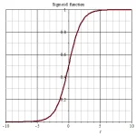
- As x → +∞, f(x) → 1.
- As x → −∞, f(x) → 0.
- At x = 0, f(0) = 0.5.

Sigmoid logistic curve showing the characteristic S-shape between 0 and 1
The smoothness of this curve is key: the sigmoid’s derivative exists at every point, allowing gradients to be computed and network weights adjusted during training. Move across the interactive plot above to see how the slope (the derivative) approaches zero at the extremes and peaks at 0.25 when x = 0.
Implementation in neural networks
In a neural network, the sigmoid is applied to each neuron’s weighted input sum:
- Compute z = w₁x₁ + w₂x₂ + … + b (weighted sum + bias).
- Apply sigmoid: a = σ(z).
- Output a feeds the next layer or is the final prediction.
During training, the sigmoid participates in gradient calculation. Its derivative is σ'(x) = σ(x)(1 − σ(x)), an elegant expression computed directly from the already-evaluated output, without re-evaluating the function.

Symbolic representation of a neuron with sigmoid activation function
Advantages and disadvantages
Advantages:
- Output interpretable as a probability between 0 and 1.
- Differentiable at every point: compatible with backpropagation.
- Monotonically increasing: ordering relationships are preserved.
Disadvantages:
- Saturation: for |x| > 5, the function flattens and the gradient approaches zero.
- Vanishing gradient: in deep networks, gradients are multiplied layer by layer and die out before reaching early layers.
- Non-zero-centred output: all outputs are positive, which can slow convergence.
These problems motivated the development of ReLU for hidden layers and the step function for conceptual analysis of binary activations.
Practical use cases
The sigmoid remains the preferred choice in specific scenarios:
- Binary classification output layer: does a patient have elevated cardiac risk? Is an email spam?
- Probability modelling: conversion prediction in marketing campaigns, credit scoring.
- Gates in LSTM architectures: memory cells use sigmoid to control what information to retain or discard.
- Logistic regression: the sigmoid is the mathematical core of one of the most widely used statistical models in industry.
An applied example: in image analysis systems, the output layer of a binary classifier (does this X-ray contain a lesion?) almost always uses sigmoid. For multi-class classification, the alternative is softmax.
The sigmoid also appears in the context of reinforcement learning, where stochastic policies sometimes produce action probabilities through this function. And in pretrained language models, classification heads inherit this pattern.
Conclusion
The sigmoid function remains irreplaceable in the output layer of any binary classifier that needs to produce an interpretable probability. Its limitations in deep layers are real but well understood: using it where appropriate and delegating to ReLU or tanh where it doesn’t belong is the key to solid neural network design.
Frequently asked questions
Why is the sigmoid no longer used in the hidden layers of deep networks?
Because for |x| > 5 its gradient drops below 0.01, and in a network with many layers, those small gradients multiply together during backpropagation until they vanish. ReLU avoids that problem because its gradient stays constant (1) for any positive input.
What is the difference between the sigmoid and the softmax function?
The sigmoid computes an independent probability per neuron, between 0 and 1, with no relationship between outputs. Softmax normalizes several outputs so they sum to 1, which is why it is used for multi-class classification; the sigmoid is reserved for binary classification or for activations that do not compete with each other, such as the gates in an LSTM.
What is the maximum value of the sigmoid’s derivative?
0.25, reached exactly at x = 0. That low ceiling is the direct mathematical cause of the vanishing-gradient problem: each additional sigmoid layer multiplies the gradient by at most 0.25.
Sources: Stanford’s CS231n course notes on activation functions[1], Deep Learning (Goodfellow, Bengio, and Courville), the feedforward-network chapter[2], and the official PyTorch documentation for torch.nn.Sigmoid[3].