Ensemble Learning in Machine Learning

Table of contents
- Key takeaways
- Bagging: parallel training on subsamples
- Boosting: sequential error learning
- Stacking: a metamodel over base predictors
- Model diversity: the necessary condition
- Evaluation and validation
- Interpretability: the ensemble cost
- Conclusion
- Frequently asked questions
- When should I use bagging versus boosting on tabular data?
- Why does my stacking ensemble look great in training but fail on new data?
- How do I know whether adding another model will actually improve the ensemble?
- Sources
Ensemble methods are the reason why winning Kaggle models almost always combine multiple predictors rather than using a single one. The intuition: if one model makes errors on certain patterns, another model can compensate, as long as the errors are not correlated.
Key takeaways
-
An ensemble combines the predictions of multiple models to obtain a more accurate and stable result than any individual model.
-
The three main paradigms are bagging (parallel training on subsamples), boosting (sequential training that corrects errors), and stacking (a metamodel learns to combine base predictors).
-
Random Forest (bagging of trees) and XGBoost/LightGBM (tree boosting) are the reference point on tabular data.
-
Diversity between models is the necessary condition for the ensemble to outperform its components.
-
The main cost is interpretability: an ensemble is always harder to explain than a single decision tree.
Bagging: parallel training on subsamples
Bootstrap Aggregating (bagging) generates multiple training-set versions through sampling with replacement (bootstrap), trains an independent model on each subsample, and combines predictions: by majority vote for classification, by averaging for regression.
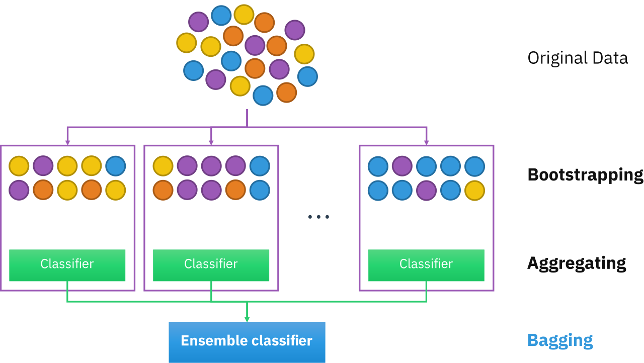 Bagging diagram: multiple bootstrap subsamples generate independent models combined via voting or averaging in the final prediction (Image: Sirakorn, CC BY-SA 4.0, via Wikimedia Commons)
The key to bagging is that the ensemble’s variance is lower than each individual model’s, as long as the models have decorrelated errors. Each model sees a slightly different view of the data; averaging cancels out the individual quirks.
Random Forest is the canonical implementation: a forest of decision trees, each trained on a dataset bootstrap and with a random subset of features available at each split. Leo Breiman formalized it in 2001, combining bagging with this extra randomness in the features at each split. The double layer of randomness, data and features, maximizes diversity between trees.
Properties of Random Forest:
-
It resists overfitting better than a single deep decision tree.
-
It reports variable importance as a byproduct of training.
-
It parallelizes: each tree trains independently.
-
It performs well even with default hyperparameters.
Boosting: sequential error learning
Boosting trains models sequentially, where each new model focuses on the examples the previous ones misclassified. The final ensemble is a weighted sum of all models. The first boosting algorithm with theoretical guarantees, AdaBoost, was published by Freund and Schapire in 1997; today the dominant variant is gradient boosting.
The general process:
-
Train a weak model (a shallow tree, for example) on the full dataset.
-
Compute the residual error: the difference between the prediction and the true value.
-
Train the next model to predict that residual.
-
Add the new model to the ensemble, with a learning rate that scales its contribution.
-
Repeat until reaching the defined number of estimators or until validation error stops improving.
XGBoost, LightGBM, and CatBoost are the most widely used implementations. Their main differences lie in the tree-construction strategy, how they handle missing values, and computational efficiency, but all of them share the gradient-boosting paradigm. XGBoost’s impact on competitions was immediate: according to the original paper by Chen and Guestrin (2016), 17 of the 29 winning solutions published on Kaggle’s blog during 2015 already used XGBoost.
In tabular-data machine learning competitions, gradient-boosting models dominate consistently.
Stacking: a metamodel over base predictors
Stacking takes the idea one step further: instead of combining models with fixed rules (voting, averaging), it trains a metamodel that learns to combine the base models’ predictions optimally.
Typical stacking process with k-fold:
-
Split the dataset into k folds.
-
For each fold: train the base models on the remaining k-1 folds, predict on the current fold.
-
Use the base models’ out-of-fold predictions as features for the metamodel.
-
Train the metamodel on these predictions.
The metamodel learns which base models are more reliable for which kinds of examples. A classic combination for tabular data: Random Forest + XGBoost + logistic regression as base learners, with LightGBM as the metamodel.
The most cited production case of stacking is the Netflix Prize. In 2009, the team BellKor’s Pragmatic Chaos won the 1,000,000 $ prize by combining hundreds of models through a stacking layer over the base predictions.
Model diversity: the necessary condition
The necessary condition for the ensemble to outperform its components is diversity. If every base model makes the same mistakes, averaging them does not help.
Sources of diversity:
-
Algorithm diversity: combining models with different inductive biases (trees, neural networks, linear regression, SVM).
-
Data diversity: bagging and its variants (pasting, random patches, random subspaces).
-
Hyperparameter diversity: the same algorithms with different configurations.
-
Feature diversity: models trained on different subsets of variables.
To evaluate diversity, the correlation matrix between the base models’ predictions is the most direct indicator: high correlation signals little additional diversity.
Evaluation and validation
Standard evaluation methods apply to the ensemble, but there is a common trap worth watching for.
Data leakage in stacking: if the metamodel trains on in-sample predictions from the base models, instead of out-of-fold ones, it learns patterns from overfitting rather than real generalization. Nested cross-validation is the correct way to evaluate the full chain.
Ensemble over-optimization: adding more base models does not always improve performance, and it always increases computational cost. Marginal returns tend to shrink.
The connection with federated learning and privacy is relevant here. In scenarios where data cannot be centralized, each participant trains its own model. The central server can then use ensemble techniques to combine the local models while preserving privacy.
Interpretability: the ensemble cost
A single decision tree is fully interpretable: you can follow the path of any prediction from the root to the leaf. An ensemble of 500 trees is not. This tension between performance and interpretability is fundamental in high-stakes domains.
Techniques that ease the problem:
-
Feature importance from Random Forest or XGBoost: shows which variables contribute most to overall predictive power.
-
SHAP values: break down each individual example’s prediction into per-feature contributions. It is the current standard for explaining ensembles.
-
Partial Dependence Plots (PDP): show a feature’s marginal effect on the prediction, averaged over the dataset.
See AI explanation through XAI for the broader context of interpretability in complex models.
Conclusion
Ensemble methods are the most mature and proven technology in classical machine learning for tabular data. Bagging reduces variance, boosting reduces bias, and stacking combines the best of multiple approaches. The condition for them to work is diversity: models that fail differently complement each other; models that fail the same way only add noise.
This article is also available in Spanish: Ensamble de aprendizaje en ML.
Sources:
- Leo Breiman, Random Forests (Machine Learning, 2001)[1]
- Chen and Guestrin, XGBoost: A Scalable Tree Boosting System (2016)[2]
- scikit-learn, Ensembles: Gradient boosting, random forests, bagging, voting, stacking[3]
- Wikipedia, Netflix Prize[4]
Frequently asked questions
When should I use bagging versus boosting on tabular data?
Bagging reduces variance: it trains independent models in parallel on bootstrap subsamples and combines them by vote or average. So Random Forest resists overfitting better than a single deep tree, parallelizes and performs well even with default hyperparameters. Boosting reduces bias: it trains shallow trees sequentially, each fitting the residual error of the previous ones, scaled by a learning rate. On tabular data, gradient boosting with XGBoost, LightGBM or CatBoost dominates competitions consistently.
Why does my stacking ensemble look great in training but fail on new data?
Most likely data leakage: if the metamodel trains on in-sample predictions from the base models instead of out-of-fold ones, it learns their overfitting rather than real generalization. The correct process splits the dataset into k folds, trains the base models on k-1 folds, predicts on the held-out fold and feeds only those out-of-fold predictions to the metamodel. Nested cross-validation is the right way to evaluate the whole chain.
How do I know whether adding another model will actually improve the ensemble?
Check diversity first: the necessary condition for an ensemble to beat its components is that the base models make different mistakes. The most direct indicator is the correlation matrix between their predictions; high correlation means little additional diversity. Diversity comes from different algorithms, data subsamples, hyperparameters or feature subsets. Adding more base models does not always improve performance, always raises computational cost, and marginal returns shrink.