Predictive Maintenance with Classic Machine Learning

Actualizado: 2026-05-03

Predictive maintenance — predicting equipment failures before they happen — is one of the Industry 4.0 applications with the clearest measurable ROI. Most successful projects don’t use deep learning. They use well-designed classic machine learning: random forests, SVMs, survival models. Understanding why helps avoid the “everything with neural networks” trap.

Key takeaways

• Typical industrial equipment (motor, pump, compressor) produces vibration, temperature, pressure, and power-consumption signals enabling three formulations: binary classification, regression, and survival models.
• 80% of success lies in feature engineering, not in the chosen algorithm.
• Random forests on extracted physical features typically beat CNNs on raw series.
• The production pipeline can run on ~50 MB RAM on an edge gateway without a GPU.
• Deep learning only adds differential value with unstructured sensors, massive fleets, or cross-plant transfer learning.

The typical problem

Industrial equipment (motor, pump, compressor) has sensors measuring vibration, temperature, pressure, and electrical consumption. The central question: when will it fail? Three formulations:

• Binary classification: “will it fail in the next week?”
• Regression: “how many days until the next failure?”
• Survival: “what’s the cumulative failure probability over time?”

Each formulation requires different treatment, but all are solved without deep learning in most cases.

Why classic ML wins here

Three reasons deep learning isn’t the first answer:

• Limited data volume. An industrial plant has perhaps 50-500 pieces of equipment with failure history. Deep learning needs thousands of labelled examples to shine; with 200 documented failures, a random forest generalises better.
• Interpretability. The maintenance operator asks “why do you think it’s going to fail?”. Random forest features are directly interpretable (“vibration increase in 120-200 Hz band”). A neural network is an oracle.
• Edge infrastructure. Models typically run on plant controllers, not in cloud. A decision tree takes kilobytes and runs in microseconds; a neural network requires GPU or dedicated acceleration.

Feature engineering: what really matters

80% of a predictive maintenance model’s success is in features, not the algorithm. Useful features extractable from vibration signals:

• Time-domain statistics: mean, variance, skewness, kurtosis, RMS value, crest factor.
• Frequency domain: energy in specific bands via FFT + integration. Defective bearings introduce characteristic frequencies.
• Hilbert envelope: classic technique for extracting high-frequency modulation, useful for incipient defects.
• Ratios and trends: current vibration divided by the healthy-equipment baseline, growth slope over the last 30 days.

A random forest on these well-extracted features typically beats a CNN on raw series — because CNNs have to relearn what we already know from physics.

Survival models

For equipment where “time to failure” is the relevant metric, survival models beat binary classification:

• Cox proportional hazards: biostatistics classic, works well here. Assumes features proportionally adjust base risk.
• Random Survival Forests: random forest extension for censored data (equipment that hasn’t failed yet).
• Weibull Accelerated Failure Time: assumes parametric distribution of time to failure; useful when reliability assumptions are well founded.

Libraries like lifelines^[1] and scikit-survival^[2] make these models accessible with APIs familiar to scikit-learn users.

Realistic production deployment

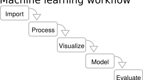
A typical production pipeline has these steps:

1. Edge gateway at the plant receives sensor data via Modbus/OPC-UA/MQTT.
2. Local aggregation: extracts features every 5-15 minutes in a sliding window.
3. Local inference with a pre-trained model (ONNX format or serialised joblib).
4. Alert to SCADA/CMMS when failure probability exceeds threshold, with inspection recommendation.
5. Feedback loop: logs whether failure occurred and feeds monthly retraining.

This flow runs on ~50 MB RAM at the edge, requires no GPU, and is fully auditable.

When deep learning does pay off

Cases where deep learning beats classic ML:

• Unstructured sensors: thermographic camera images or high-frequency continuous vibration audio. CNNs and RNNs extract patterns where feature engineering is more costly than training the network.
• Massive volumes: 10,000+ equipment fleet with continuous telemetry. Deep learning scales; random forest starts saturating memory.
• Transfer learning between plants: a model pre-trained on one fleet can adapt with less data from another. Hard to replicate with trees.

But these cases are the minority. 80% of predictive maintenance projects are solved with well-done classic ML.

Also see our coverage of the Industry 4.0 revolution and industrial digital twins — the broader context where predictive maintenance makes sense.

Conclusion

The deep learning hype tends to obscure that predictive maintenance is a well-solved problem with classic techniques. Teams adopting classic ML first get value earlier, with lower investment in data and infrastructure, and with models plant personnel understand. Deep learning is reserved for genuinely complex cases.

1. lifelines
2. scikit-survival