Momentum in Gradient Descent
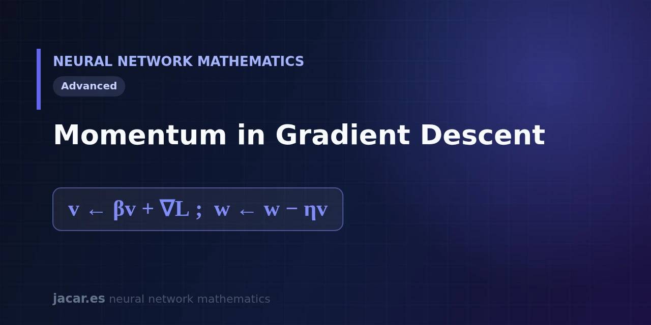
Table of contents
Momentum adds memory to gradient descent: instead of moving with the current step’s gradient alone, it accumulates a velocity that keeps the direction of previous steps. That inertia, borrowed from the physics of a rolling ball, smooths the zigzag of stochastic gradient descent and speeds up the arrival at the minimum. The idea comes from Boris Polyak, who proposed it in 1964, and it remains the basis of modern optimisers such as Adam.
This guide explains the rule $\mathbf{v}\leftarrow\beta\mathbf{v}+\nabla L$, the role of the coefficient $\beta$ and when momentum makes a difference over plain SGD. The same explanation is available in Spanish.
Key takeaways
- Momentum keeps an accumulated velocity
vthat combines past gradients with the current one, instead of reacting only to the slope of the moment. - The update happens in two steps:
v ← βv + ∇Lto accumulate the velocity andw ← w − ηvto move the weights with that velocity. - The coefficient
β, whose default value is 0.9, decides how much memory we keep: with 0.9 each gradient carries weight for about ten steps before fading out. - Momentum pushes through the long narrow valleys and plateaus where stochastic gradient descent crawls, because the useful gradient components add up step by step.
- It is the seed of optimisers such as Nesterov and Adam, which in 2014 combined momentum with an adaptive learning rate and became the default method of deep learning.
What momentum is
Basic gradient descent corrects the weights by looking only at the slope where it stands: it computes the gradient ∇L, takes a step in the opposite direction and forgets everything before. That amnesia is its weak point. When the error surface is a narrow, elongated valley, the gradient points mostly toward the walls, not toward the floor, and the method bounces from side to side while making little progress.
Momentum solves that by giving the process memory. Rather than using the raw gradient, it keeps a velocity v that updates by adding the new gradient to a fraction of the previous velocity. Directions that repeat reinforce each other and those that oscillate cancel out.
The result is a straighter, faster move toward the minimum. This method builds on classic gradient descent and only changes how each step is computed.
The rolling ball analogy
The usual image is a heavy ball rolling down the error surface. Pure gradient descent behaves like a massless marble: at every instant it goes exactly where the slope points and stops as soon as the ground flattens. A ball with mass, by contrast, has inertia: if it has been descending in one direction for a while, it keeps going that way even when the terrain shifts a little.
That inertia is precisely what momentum contributes. In a narrow valley, the heavy ball does not bounce between the walls; its accumulated velocity pushes it along the floor toward the minimum. On an almost flat plateau, where a marble would stall, the ball keeps part of the velocity it carried and keeps rolling. This is why Polyak’s original version is known as the heavy ball method.
The accumulated velocity formula
Mathematically, momentum adds a single variable, the velocity $\mathbf{v}$, and rewrites the update in two steps:
$$\mathbf{v}\leftarrow\beta\mathbf{v}+\nabla L,\qquad \mathbf{w}\leftarrow\mathbf{w}-\eta\mathbf{v}$$
In pseudocode, the training loop looks like this:
v = 0                       # initial velocity
for step in training:
    grad = gradient(L, w)   # gradient of the loss at w
    v = beta * v + grad     # accumulate the velocity
    w = w - eta * v         # move the weights with that velocity
The first line, $\mathbf{v}\leftarrow\beta\mathbf{v}+\nabla L$, is the heart of the method: the new velocity is a part of the previous velocity (the $\beta\mathbf{v}$ term) plus the freshly computed gradient. The second, $\mathbf{w}\leftarrow\mathbf{w}-\eta\mathbf{v}$, is the usual update, except that we now use the velocity $\mathbf{v}$ instead of the bare gradient. If you set $\beta=0$, the velocity collapses to the gradient and you recover exactly classic gradient descent; momentum is a generalisation that contains it as a special case. This block fits into the mathematics behind neural networks roadmap, within optimisation.
The added cost of momentum is minimal: a single state variable per weight, the velocity $\mathbf{v}$, and one extra multiplication per step, without touching the loss function or the gradient computation.
The beta coefficient
The coefficient $\beta$ controls how much memory the velocity keeps, and it is almost always set between 0.9 and 0.99. Its effect follows from a simple count: with geometric memory, each gradient influences roughly $1/(1-\beta)$ steps. With $\beta=0.9$ that is about 10 steps of effective history; with $\beta=0.99$, about 100. The larger $\beta$ is, the longer the memory and the smoother (but also lazier) the trajectory.
Show the derivation
Unrolling the recurrence $\mathbf{v}_t=\beta\mathbf{v}_{t-1}+\mathbf{g}_t$, a single step’s gradient $\mathbf{g}_k$ contributes to later steps with weights $1,\beta,\beta^2,\dots$ Its total influence is the geometric sum $\sum_{i=0}^{\infty}\beta^i=\frac{1}{1-\beta}$, and the effective time it carries weight before fading is exactly $1/(1-\beta)$ steps. With $\beta=0.9$ that gives $10$; with $\beta=0.99$, $100$.
Choosing $\beta$ well is a trade-off. A value that is too high, such as 0.999, accumulates so much inertia that the ball overshoots the minimum and is slow to brake. One that is too low barely helps over stochastic gradient descent.
In practice, $\beta=0.9$ is the starting point recommended in almost every textbook, and it is only raised to 0.99 when the gradient is noisy and more averaging pays off. As Sebastian Ruder puts it in his overview of optimisation algorithms[1], «the momentum term increases for dimensions whose gradients point in the same directions and reduces updates for dimensions whose gradients change directions».
Momentum versus plain SGD
The practical difference shows up in two common situations. The first is elongated valleys, where plain stochastic gradient descent makes a slow zigzag between the walls. With momentum, the lateral gradient components cancel between consecutive steps while the component toward the floor adds up, so the trajectory straightens and training converges in far fewer epochs. The interactive article Why Momentum Really Works[2], published in Distill in 2017, shows visually how that accumulation reduces the oscillations.
The second situation is plateaus and shallow local minima. The accumulated velocity acts as an energy reserve that helps cross almost flat regions and climb out of small pits where plain descent would get stuck. The cost is minimal: one extra variable per weight and one more multiplication per step.
In return, momentum applies just as well to batch, stochastic and mini-batch gradient descent, whatever the batch size the gradient is estimated on. The Wikipedia page on stochastic gradient descent[3] lists momentum among its most-used extensions.
Frequently asked questions
How does momentum differ from plain SGD?
Momentum keeps an accumulated velocity instead of using only the current step’s gradient. Plain stochastic gradient descent corrects the weights with w ← w − η∇L and forgets each step; momentum inserts v ← βv + ∇L first, so the direction of previous steps keeps influencing the move. That inertia reduces the zigzag and speeds up convergence without changing the loss function.
What value of beta should I use?
The usual starting point is β = 0.9, which is like remembering about ten steps of gradient. If the gradient is noisy, raising it to 0.99 averages more history and stabilises the trajectory; dropping below 0.9 leaves the method close to ordinary stochastic gradient descent. It is rarely pushed past 0.99, because excessive inertia makes the model overshoot the minimum.
Does momentum work with mini-batch?
Yes, and that is exactly where it is used most. With mini-batch each gradient is a noisy estimate, and momentum averages them over the window of steps its coefficient β sets, which filters out much of that noise. Almost all modern training combines mini-batch with momentum, or directly with Adam, which integrates momentum as one of its two ingredients.
Conclusion
Momentum turns gradient descent into a process with inertia: it accumulates a velocity v ← βv + ∇L and moves the weights with it through w ← w − ηv. With a coefficient β of 0.9 it filters noise, straightens the trajectory in elongated valleys and crosses the plateaus where plain SGD stalls, all for one extra variable per weight. The natural next step is to see how Adam combines this idea with an adaptive learning rate, inside the mathematics behind neural networks roadmap.