Batch, Stochastic and Mini-Batch Gradient Descent
Table of contents
Updated: 2026-10-19
Gradient descent comes in three variants depending on how much data you use to compute each step: batch (all of it), stochastic (one sample) and mini-batch (an intermediate group). The update rule is the same in all three, $\mathbf{w} \leftarrow \mathbf{w}-\eta\cdot\nabla L$, but the number of examples that enters that gradient completely changes the speed, the memory and the noise of training. This guide compares the three options, explains where the noise comes from and why mini-batch with batches of 32 to 256 samples has become the standard. The same explanation is available in Spanish.
Key takeaways
- Batch gradient descent computes the gradient over the whole training set before taking a step: accurate but slow and heavy on memory.
- Stochastic gradient descent (SGD) updates the weights after every single sample: a thousand times more steps, plenty of noise and a zigzag path toward the minimum.
- Mini-batch averages the gradient over a small group of 32 to 256 examples, and combines the best of the two previous ideas.
- The batch size is a hyperparameter: small batches add noise and generalise better; large batches converge smoothly but may settle into worse minima.
- The noise is not merely a flaw: it helps escape shallow local minima, which is why SGD and mini-batch generalise better than pure batch descent.
Batch gradient descent
Batch gradient descent is the textbook version. On each iteration it goes through the $N$ samples of the training set, computes the average gradient of the loss and takes a single step: $\mathbf{w} \leftarrow \mathbf{w}-\eta\cdot\nabla L_{\text{batch}}$. As the book Deep Learning[1] by Goodfellow, Bengio and Courville puts it, this full gradient is the most faithful estimator of the descent direction, because it averages the error over all available data.
The problem is the cost. If you have 50,000 examples, each step forces you to process all 50,000 before moving a single weight. With sets of millions of samples that becomes unworkable: one update would take minutes and the whole set might not fit in memory.
The path to the minimum is smooth and direct, but you take very few steps per hour. For today’s large problems that smoothness is too expensive. This rule is the same one we saw in partial derivatives and the gradient; here we only decide how much data it is averaged over.
Stochastic gradient descent (SGD)
Stochastic gradient descent goes to the other extreme: it uses a single randomly chosen sample to estimate the gradient and updates the weights immediately. With 50,000 examples, one full pass over the data (an epoch) produces 50,000 updates instead of one. The model starts improving from the first instant, without waiting to see the entire set.
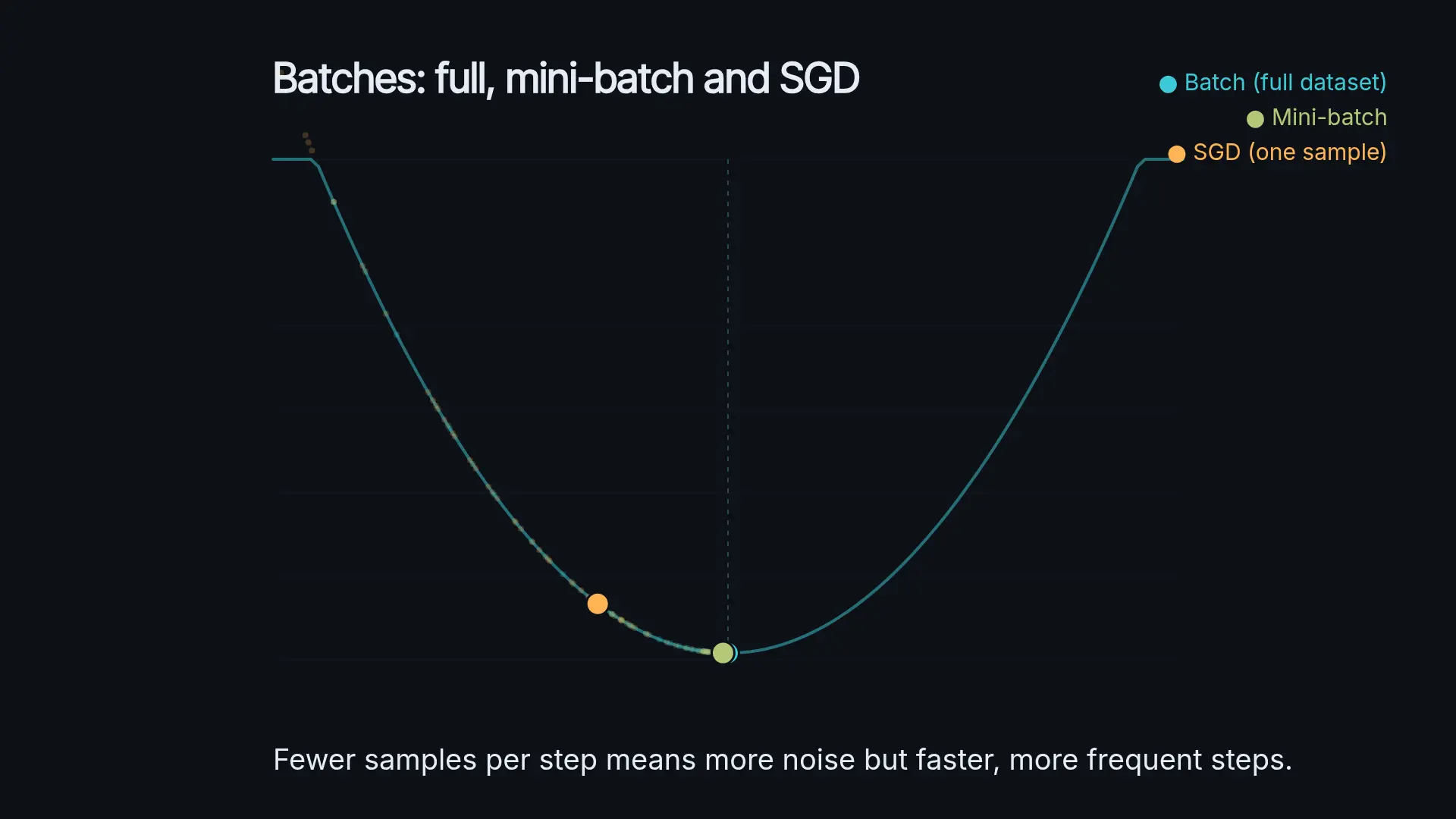
The price is noise. The gradient of a single sample is a rough estimate of the true gradient, so the path to the minimum zigzags constantly instead of forming a clean line. That wobble has an unexpected benefit: the jolts help jump out of shallow local minima, something that batch descent, being too orderly, cannot manage.
The word "stochastic" means exactly that, that we inject randomness into the process. The Wikipedia page on stochastic gradient descent[2] records the history of the method, which traces back to the Robbins-Monro rule of 1951.
Mini-batch, the practical balance
Mini-batch is the middle ground, and the one almost every real system uses. Instead of one example or all of them, we take a small group (the batch) and average its gradient before updating. With a batch of 128 samples over 50,000 examples, an epoch gives about 390 updates: far more than batch descent, far less noisy than pure SGD.
This balance has two practical advantages. First, the gradient averaged over 32 or 128 samples is much more stable than the one from a single example, so convergence is cleaner. Second, and decisively, batches fit the hardware beautifully: a GPU multiplies all the samples of the batch in parallel, using the same matrix computation behind the mathematics of neural networks.
That is why, when someone says "SGD" today, they almost always mean mini-batch. Sebastian Ruder’s reference guide on gradient descent optimization[3] treats the three variants under that same umbrella.
The batch size
The batch size is the hyperparameter that governs this whole balance, and it is almost always chosen between 32 and 256, in powers of two to align with GPU memory. It is not a magic number but a trade-off.
Small batches (16, 32) inject more noise into each step, use little memory and, curiously, tend to generalise better: the noise acts as a soft regularisation.
Large batches (512, 1,024 or more) give stable gradients and use the GPU better per step. But they need a lot of memory and tend to fall into "sharp" minima that generalise worse on new data. On this point, Yann LeCun summed up the field’s intuition with a famous line: «training with large minibatches is bad for your health; more importantly, it is bad for your test error; friends do not let friends use minibatches larger than 32». The exact figure is debated, but the direction is clear: when in doubt, start small.
Noise and convergence
The word that connects the three variants is noise, and it pays to understand it well. The "true" gradient is the one from batch descent; any estimate with less data adds random error. SGD has the most noise (one sample), mini-batch an intermediate amount and batch descent none.
That noise changes how convergence looks. With SGD or mini-batch, the loss does not fall perfectly monotonically: it oscillates as it descends. Near the minimum it keeps circling within a small region rather than stopping at the exact point. To fine-tune the ending, the standard approach is to reduce the learning rate $\eta$ over time (a learning rate schedule), so the jumps shrink once we are close.
The basic rule $\mathbf{w} \leftarrow \mathbf{w}-\eta\cdot\nabla L$ is still the same as always; the only thing that changes between batch, sample and mini-batch is how many examples that $\nabla L$ is estimated on.
When people say “SGD” today they almost always mean mini-batch: the update $\mathbf{w} \leftarrow \mathbf{w}-\eta\cdot\nabla L$ is applied to the gradient averaged over a batch, not over a single sample.
Frequently asked questions
How do batch, SGD and mini-batch differ?
In how many samples they use to estimate each gradient. Batch descent uses the whole training set, stochastic gradient descent uses a single sample and mini-batch uses an intermediate group of 32 to 256 examples. The update rule $\mathbf{w} \leftarrow \mathbf{w}-\eta\cdot\nabla L$ is identical in all three; only the size of the sample it is averaged over changes.
What batch size should I use?
As a starting point, a value between 32 and 256, in powers of two to make the most of GPU memory. If your model generalises poorly, try lowering the batch to add more noise; if training is slow and you have memory to spare, raise it. There is no universal optimum: it depends on the model, the data and the hardware.
Why can the noise in SGD be beneficial?
Because the oscillations help jump out of shallow local minima and saddle points where a noise-free method would get stuck. That same noise also acts as a soft regularisation that improves generalisation, and it is one of the reasons mini-batch beats pure batch descent in practice.
Conclusion
Batch gradient descent is accurate but slow, the stochastic version is fast but noisy, and mini-batch balances both with batches of 32 to 256 samples that fit the GPU. The rule $\mathbf{w} \leftarrow \mathbf{w}-\eta\cdot\nabla L$ does not change; what you decide is how much data you compute that step on. The natural next step is to see how the step itself is refined with methods such as momentum and Adam, inside the mathematics behind neural networks roadmap.
Sources: [1] Deep Learning (Goodfellow, Bengio and Courville)[1], [2] An overview of gradient descent optimization algorithms (Sebastian Ruder)[3], [3] Stochastic gradient descent (Wikipedia)[2].