Nesterov Accelerated Gradient (NAG)
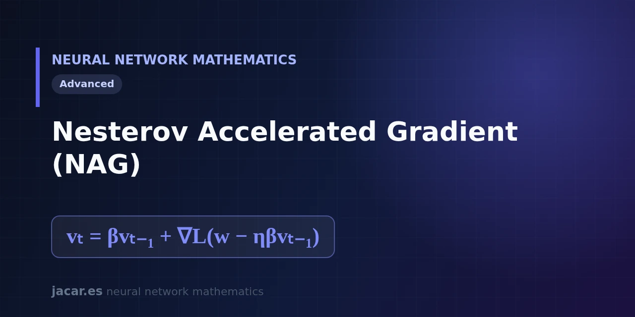
Table of contents
- Key takeaways
- What Nesterov improves over momentum
- The look-ahead step
- The formula
- The convergence advantage
- Nesterov versus classic momentum
- Frequently asked questions
- How does Nesterov differ from classic momentum?
- What value of β should I use?
- Does Nesterov always converge faster?
- Conclusion
- Sources
Nesterov accelerated gradient looks one step ahead before deciding where to go. Classic momentum builds up inertia and evaluates the gradient at the current position; Nesterov evaluates that gradient at the point inertia is about to reach. That small change of order turns inertia into a self-correcting force that brakes before overshooting, and it speeds up convergence with no appreciable extra cost. This guide is part of the mathematics behind neural networks roadmap, and the same explanation is available in Spanish.
Key takeaways
- Nesterov accelerated gradient (NAG) evaluates the gradient at a look-ahead point, $w-\eta\beta v$, instead of at the current point $w$.
- That look-ahead step acts as a correction: it brakes before overshooting when inertia points the wrong way.
- Yurii Nesterov introduced it in 1983 with an $O(1/k^2)$ convergence guarantee for smooth convex functions, versus the $O(1/k)$ of plain gradient descent.
- For strongly convex functions, NAG cuts the iteration count from a factor proportional to the condition number $\kappa$ to one proportional to its square root $\sqrt{\kappa}$.
- In practice it uses a momentum coefficient $\beta$ around 0.9 and shares almost all its code with classic momentum.
What Nesterov improves over momentum
Classic momentum, proposed by Boris Polyak in 1964 and known as the heavy-ball method, adds inertia to gradient descent. At each iteration it accumulates a velocity $v$ that blends the new gradient with the previous direction, so it crosses flat regions faster and damps the oscillations in narrow valleys.
Its weakness is that it decides the step by looking only at where it is now. If the accumulated inertia already points toward a region where the terrain changes, classic momentum does not know until it arrives, and by then it has already overshot. Nesterov fixes exactly that: it first takes the jump inertia dictates and only then measures the slope, so the gradient already reflects the terrain of the destination rather than the origin.
The look-ahead step
The intuition is this. Before computing the gradient, Nesterov moves the weights to the point inertia is going to visit anyway, $w-\eta\beta v$, and measures the slope there. That look-ahead point is a glimpse into the immediate future of the trajectory.
When the look-ahead reveals that the descent is about to overshoot, the gradient at that point points backward and slows the velocity before the error accumulates. As Sebastian Ruder puts it in his overview of optimisation methods, «Nesterov accelerated gradient (NAG) is a way to give our momentum term this kind of prescience». That foresight is what avoids the more violent oscillations of classic momentum.
The formula
Starting from the velocity $v$, the learning rate $\eta$ and the momentum coefficient $\beta$, each NAG iteration reads:
$$vt = \beta v{t-1} + \nabla L(w-\eta\beta v_{t-1})$$
$$w = w-\eta v_t$$
The first line evaluates the gradient at the look-ahead point $w-\eta\beta v_{t-1}$ and the second updates the weights with the already-corrected velocity. Compare the second piece with classic momentum, which evaluates $\nabla L(w)$ at the current point. The only change is the argument of the gradient: $w-\eta\beta v$ instead of $w$. The learning rate $\eta$ still controls the step size, and $\beta$ weighs how much inertia carries over from one iteration to the next.
Modern libraries implement a rewrite of it, the Sutskever and Bengio form popularised in 2013, which avoids recomputing the weights at two separate points and is algebraically equivalent to this one.
The convergence advantage
The reason Nesterov matters is not only empirical. For a smooth convex function (with Lipschitz gradient), gradient descent reduces the error at a rate of $O(1/k)$ after k iterations. Nesterov’s method lowers it to $O(1/k^2)$: with 100 iterations, the error bound goes from scaling like 1/100 to scaling like 1/10,000.
That $O(1/k^2)$ is not an ordinary improvement. Nesterov proved it is the optimal speed any method using only first-order gradients can reach on this class of problems, so there is no room to do better without extra information. For strongly convex functions the iteration count goes from proportional to $\kappa$, the condition number, to proportional to $\sqrt{\kappa}$. If $\kappa$ is 10,000, the square root brings it down to 100.
The $O(1/k^2)$ bound is a worst-case rate for smooth convex functions; on a real neural network, which is not convex, it describes a practical tendency rather than a guarantee.
Nesterov versus classic momentum
In a real neural network the loss is not convex, so the theoretical guarantees do not hold to the letter. Even so, the look-ahead intuition carries over well: NAG tends to produce more stable trajectories and to tolerate slightly larger learning rates, because the anticipated braking contains the oscillations.
The code difference is minimal. If you already have momentum, switching to Nesterov means changing the point where you evaluate the gradient, nothing more. That is why turning it on comes down to a flag, nesterov=True, and Adam folds the same idea into its Nadam variant. When classic momentum falls short because of oscillations, Nesterov is the first adjustment to try.
Frequently asked questions
How does Nesterov differ from classic momentum?
In where the gradient is computed. Classic momentum evaluates it at the current position $w$; Nesterov evaluates it at the look-ahead point $w-\eta\beta v$, the one inertia is about to reach. That anticipation lets it brake before overshooting.
What value of β should I use?
A momentum coefficient between 0.9 and 0.99 works well, and 0.9 is the default. The higher $\beta$ is, the more inertia carries over and the more valuable Nesterov’s anticipated correction becomes.
Does Nesterov always converge faster?
On smooth convex problems yes, with the $O(1/k^2)$ guarantee. On neural networks, which are not convex, the improvement is empirical and not guaranteed, although in practice its trajectories come out more stable than those of classic momentum.
Conclusion
Nesterov accelerated gradient is a rare example of an improvement that costs almost nothing. A single change in the argument of the gradient turns inertia into a self-correcting force and improves convergence from $O(1/k)$ to $O(1/k^2)$ in the convex case. It is the natural bridge between classic momentum and adaptive optimisers like Adam, and it fits into the wider mathematics behind neural networks roadmap.
Sources: [1] An overview of gradient descent optimization algorithms (Sebastian Ruder)[1], [2] Why Momentum Really Works (Distill, 2017)[2], [3] Stochastic gradient descent, Nesterov momentum (Wikipedia)[3], [4] Neural Networks Part 3, CS231n (Stanford)[4].