Second-Order Methods: Newton and Its Approximations
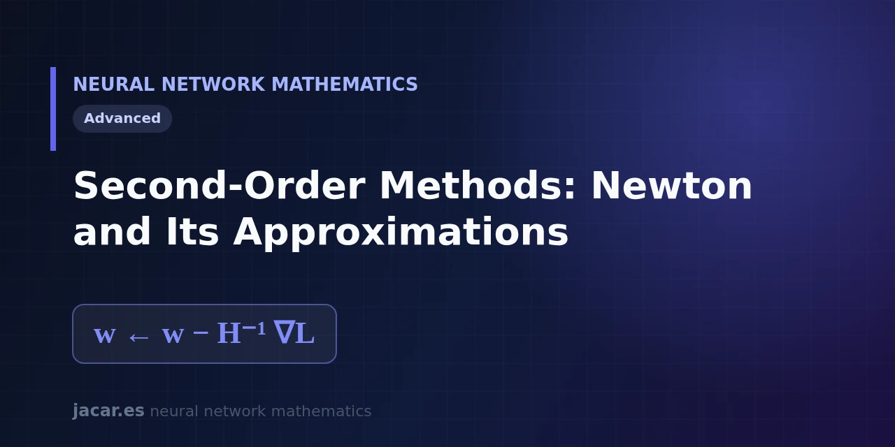
Table of contents
- Key takeaways
- The second-order information (the Hessian)
- Newton's method
- Why it is expensive in deep learning
- Quasi-Newton approximations (L-BFGS) and K-FAC
- When they are used
- Frequently asked questions
- How does Newton's method differ from gradient descent?
- Why is Newton's method not used to train large neural networks?
- How are L-BFGS and K-FAC related to Newton's method?
- Conclusion
- Sources
Second-order methods look not only at the slope of the loss but also at its curvature. Classic gradient descent uses the first derivative to know which way to go down. Second-order methods add the second derivative, gathered in a matrix called the Hessian, to know how far to step as well.
Newton’s method is the pure member of this family, and its formula $\mathbf{w} \leftarrow \mathbf{w}-\mathbf{H}^{-1}\nabla L$ promises far faster convergence. The catch is the price.
This guide explains the idea, why it becomes impractical in large networks and which approximations rescue it. The same explanation is available in Spanish.
Key takeaways
- Newton’s method updates the weights with $\mathbf{w} \leftarrow \mathbf{w}-\mathbf{H}^{-1}\nabla L$, where $\mathbf{H}$ is the Hessian and $\nabla L$ the gradient of the loss.
- The Hessian is the matrix of all second derivatives: for a network with $n$ parameters it has $n\times n$ entries.
- Near a minimum, Newton converges quadratically, much faster than gradient descent, which advances linearly.
- Building and inverting the Hessian costs on the order of $n^3$ operations, unfeasible when $n$ is billions of weights.
- Quasi-Newton approximations like L-BFGS and curvature methods like K-FAC capture part of that information at an affordable cost.
The second-order information (the Hessian)
The gradient $\nabla L$ answers one question: in which direction the loss grows fastest. That is first-order information, the slope. But a slope does not say whether the terrain curves gently or drops sharply, and that curvature is exactly what decides how far it is worth stepping. That is where the second derivative comes in.
When the loss depends on more than one weight, there is not a single second derivative but one for each pair of parameters. All of them are arranged in the Hessian, a square matrix $\mathbf{H}$ where the entry in row $i$ and column $j$ is the partial derivative of $L$ first with respect to weight $i$ and then with respect to weight $j$. Wikipedia[1] defines it precisely as the matrix of second-order partial derivatives of a scalar function.
The Hessian extends the ideas of partial derivatives and the gradient: if the gradient is a vector with $n$ components, the Hessian is a table of $n\times n$ numbers. Its values describe the local shape of the loss surface: whether it is a narrow valley, a wide valley or a saddle point. When the Hessian is positive definite, the surface curves upward in every direction and we are near a minimum.
Newton’s method
Newton’s method springs from a simple idea: approximate the loss around the current point by a parabola (a quadratic model) and jump straight to its minimum. That parabola uses the gradient for the slope and the Hessian for the curvature. Solving for its minimum yields the cover formula:
$$\mathbf{w} \leftarrow \mathbf{w}-\mathbf{H}^{-1}\nabla L$$
Show the derivation
Approximate the loss near the current point with the second-order Taylor expansion $L(\mathbf{w}+\Delta)\approx L(\mathbf{w})+\nabla L^{\top}\Delta+\tfrac{1}{2}\Delta^{\top}\mathbf{H}\Delta$. To find the minimum of that parabola we differentiate with respect to the step $\Delta$ and set it to zero: $\nabla L+\mathbf{H}\Delta=\mathbf{0}$. Solving gives $\Delta=-\mathbf{H}^{-1}\nabla L$, that is the update $\mathbf{w} \leftarrow \mathbf{w}-\mathbf{H}^{-1}\nabla L$.
Compared with gradient descent, $\mathbf{w} \leftarrow \mathbf{w}-\eta\nabla L$, the change is telling: the learning rate $\eta$, a fixed number we pick by hand, is replaced by $\mathbf{H}^{-1}$, the inverse Hessian. Instead of taking the same step in every direction, Newton stretches or shrinks the step according to the curvature of each axis. In a long, narrow valley, where gradient descent zigzags, Newton aims almost straight at the bottom.
The reward is speed. Near a minimum, Newton’s method converges quadratically: the number of correct decimals doubles at each iteration. Gradient descent, by contrast, advances linearly. With a good starting point, Newton reaches in a handful of iterations a precision that would cost the gradient hundreds.
The inverse Hessian only points downhill if $\mathbf{H}$ is positive definite, that is, if the surface curves upward in every direction. When there is negative curvature, the Newton step stops being a descent and has to be corrected with regularisation or damping.
That promise carries important fine print. As Goodfellow, Bengio and Courville warn in «Deep Learning», «Newton’s method is only appropriate when the nearby Hessian is positive definite». If the Hessian has negative curvature, common at the saddle points of the loss surface, Newton can jump upward instead of down.
Why it is expensive in deep learning
This is where theory collides with practice. The Hessian of a network with $n$ parameters has $n\times n$ entries, and that square scales terribly. A modest network with 1,000,000 parameters would have a Hessian of 1,000,000,000,000 numbers: storing it in memory is already impossible, long before touching it.
The problem does not end at storage. Newton’s method needs $\mathbf{H}^{-1}$, and computing the inverse of an $n\times n$ matrix costs on the order of $n^3$ operations. Even though in practice one does not invert the matrix but solves a linear system, the cost is still cubic. That $n^3$ factor is what makes Newton splendid for problems with hundreds of variables and unthinkable for models with millions or billions.
One example shows the scale of the wall. GPT-3 has 175 billion parameters. Its full Hessian would have on the order of $3\times10^{22}$ entries, a figure with no physical meaning: it would not fit on all the hard drives on the planet combined. That is why deep learning is almost always trained with first-order methods like gradient descent and its variants, which need only the gradient.
There is an added obstacle: noise. In deep learning the loss is estimated over minibatches of data, so both the gradient and the Hessian are noisy estimates. A noisy, indefinite Hessian can push the Newton step in the wrong direction, as the optimisation chapter of Deep Learning[2] summarises.
Quasi-Newton approximations (L-BFGS) and K-FAC
If the exact Hessian is untouchable, the way out is to approximate it. Quasi-Newton methods build an estimate of $\mathbf{H}^{-1}$ from the gradients already computed at each step, without forming the matrix. The best known is BFGS, from 1970, which keeps a dense approximation of the inverse and improves it at every iteration.
BFGS still stores an $n\times n$ matrix, so for large networks its limited-memory version, L-BFGS, is used. Instead of the full matrix, L-BFGS keeps only between 5 and 20 vectors from the recent history of gradients and positions, and with them reconstructs the effect of $\mathbf{H}^{-1}$ on the gradient. The cost per step drops to something proportional to $n$, not to $n^2$. L-BFGS works well when the gradient is precise (for instance in full batch), but struggles with minibatch noise, as Wikipedia on L-BFGS[3] describes.
For deep neural networks the most influential proposal is K-FAC (Kronecker-Factored Approximate Curvature), introduced by James Martens and Roger Grosse in 2015. K-FAC does not approximate the whole Hessian but the Fisher information matrix, and assumes it can be factored blockwise as a Kronecker product of two small matrices per layer. That trick turns one giant inversion into one tiny inversion per block, and captures the curvature between weights of the same layer at an affordable cost. The original paper is available on arXiv[4].
Both ideas share a philosophy with the book Mathematics for Machine Learning[5]: use structure so as not to pay the full price of the exact computation.
When they are used
In ordinary deep-network training, pure second-order methods barely appear. The field leans on first-order optimisers with implicit curvature, such as Adam, which adapt the step per parameter using gradient statistics without building any Hessian. They are far cheaper and tolerate minibatch noise better.
Even so, second-order information has its niches. L-BFGS is a solid choice when the problem is of moderate size and the gradient is computed over all the data. That is the case in fitting classic models, in computational physics or in image reconstruction. K-FAC and its descendants are researched to speed up the training of large networks and for reinforcement learning, where a better step direction pays back the extra computation.
The practical rule is this: if you have millions of parameters and noisy data, start with a well-tuned first-order method. Reserve second-order methods for when the curvature of the problem is the real bottleneck and you can afford to estimate it.
Frequently asked questions
How does Newton’s method differ from gradient descent?
Gradient descent uses only the first derivative and steps with a fixed size $\eta$ equal in every direction. Newton’s method adds the second derivative through the Hessian and fits the step to the curvature of each direction, replacing $\eta$ by $\mathbf{H}^{-1}$. In exchange for converging much faster near a minimum, it pays a far higher cost per iteration.
Why is Newton’s method not used to train large neural networks?
Because the Hessian of a network with $n$ parameters has $n\times n$ entries and inverting it costs on the order of $n^3$ operations. With millions or billions of weights it does not even fit in memory. Moreover, the Hessian estimated over minibatches is noisy and may not be positive definite, which would send the step in the wrong direction.
How are L-BFGS and K-FAC related to Newton’s method?
Both are approximations. L-BFGS reconstructs the effect of the inverse Hessian using between 5 and 20 vectors of past gradients, at a cost proportional to $n$. K-FAC approximates the curvature blockwise through Kronecker products per layer. Both chase part of Newton’s benefit without paying the cubic cost of the full Hessian.
Conclusion
Second-order methods provide what the gradient lacks: a sense of the curvature of the loss. Newton’s method takes that idea to the limit with the formula $\mathbf{w} \leftarrow \mathbf{w}-\mathbf{H}^{-1}\nabla L$ and quadratic convergence near the minimum, but the $n^3$ cost of the Hessian bars it from large-scale training. Quasi-Newton and curvature approximations, such as L-BFGS and K-FAC, recover part of that information at a reasonable price. The natural next step is to place these pieces inside the roadmap of the mathematics of neural networks.
Sources: [1] Deep Learning (Goodfellow, Bengio and Courville)[2], [2] Hessian matrix (Wikipedia)[1], [3] Optimizing Neural Networks with Kronecker-factored Approximate Curvature (Martens and Grosse, 2015)[4], [4] Mathematics for Machine Learning (Deisenroth, Faisal and Ong)[5].