Matrix Multiplication in Neural Networks
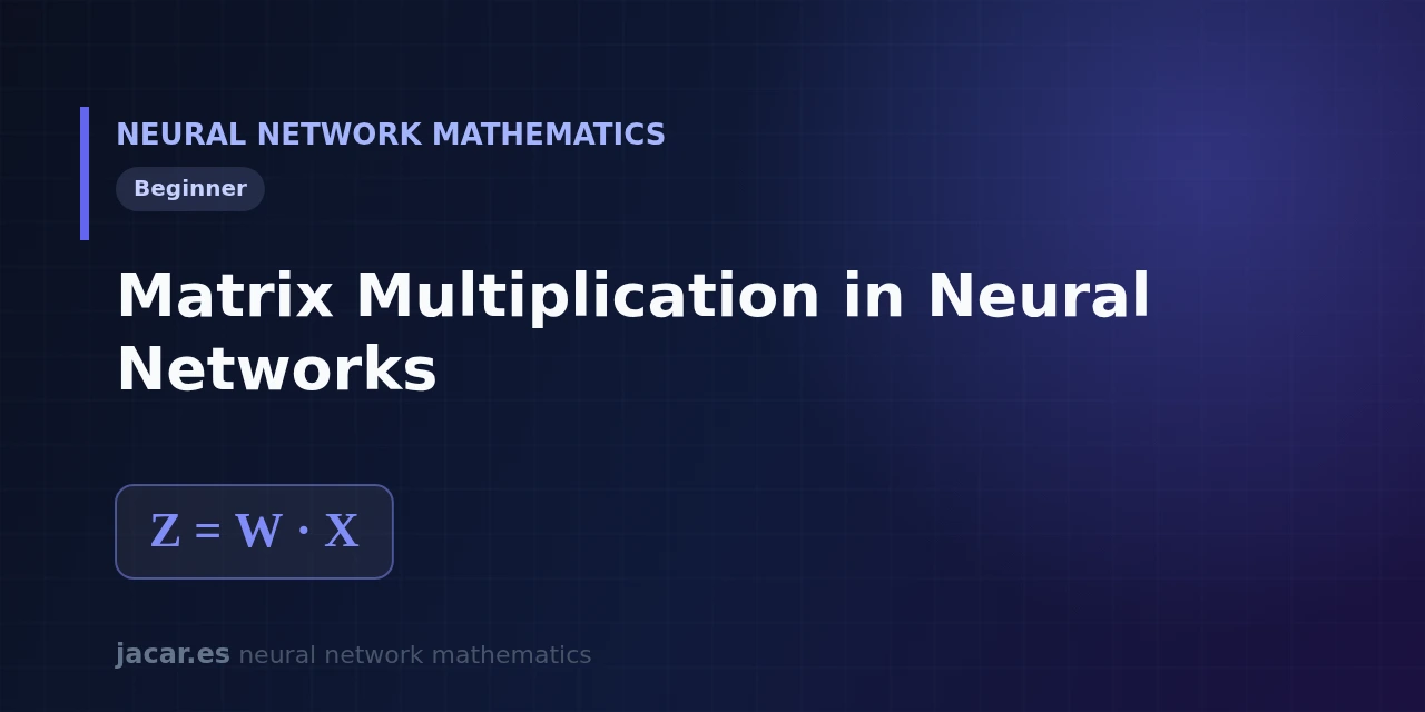
Table of contents
- Key takeaways
- Matrix multiplication rules
- Why a layer is a matrix multiplication
- Batches: processing many examples at once
- Computational cost
- Worked example
- Frequently asked questions
- What is the difference between matrix multiplication and element-wise multiplication?
- Why are GPUs so good for neural networks?
- What happens if the dimensions do not match?
- Conclusion
- Sources
Inside every layer of a neural network there is a matrix multiplication. It is the operation that combines all the inputs with all the weights at once and produces the result that flows to the next layer. Understanding that operation, its dimension rules and its cost is what it takes to really grasp how a network computes.
This guide explains it from scratch, with a worked numerical example. The same explanation is available in Spanish.
Key takeaways
- The matrix multiplication at the heart of neural networks gathers a layer’s weights into a matrix
Wand computes the output asZ = W · X. - To multiply two matrices, the number of columns of the first must match the number of rows of the second; the result inherits the rows of one and the columns of the other.
- Processing a batch of examples at once just adds columns to
X: the same weight matrix serves for 1 or for 32 examples without any change. - Multiplying an
m × nmatrix by ann × pmatrix costs about2 · m · n · poperations, and that is where roughly 90% of a network’s work happens. - A model like GPT-3, with 175 billion parameters, is nothing but billions of these multiplications chained together and run in parallel.
Matrix multiplication rules
Multiplying matrices is not multiplying element by element. The rule is different and has two parts worth fixing before we go on.
The first is the dimension rule. If $\mathbf{A} \in \mathbb{R}^{m \times n}$ (m rows, n columns) and $\mathbf{B} \in \mathbb{R}^{n \times p}$, then the product $\mathbf{A}\mathbf{B}$ exists and has shape $m \times p$:
$$\mathbf{A} \in \mathbb{R}^{m \times n},\quad \mathbf{B} \in \mathbb{R}^{n \times p} \;\Longrightarrow\; \mathbf{A}\mathbf{B} \in \mathbb{R}^{m \times p}$$
The two inner dimensions must match (the $n$) and disappear; the two outer ones ($m$ and $p$) become the result’s shape. If those inner dimensions do not agree, the operation is undefined and the program fails.
The second is how each number of the result is computed. The element in row $i$ and column $j$ of $\mathbf{A}\mathbf{B}$ is the dot product between row $i$ of $\mathbf{A}$ and column $j$ of $\mathbf{B}$:
$$(\mathbf{A}\mathbf{B}){ij} = \sum{k=1}^{n} A{ik}\,B{kj}$$
You pair them term by term, multiply and add. That dot product is the same operation we study in the dot product and the neuron. This is why a matrix times a vector is just a repeated dot product, one per row.
One important warning: order matters. $\mathbf{A}\mathbf{B}$ is not equal to $\mathbf{B}\mathbf{A}$ except in special cases, and one of the two products does not even exist when the dimensions do not fit.
In a neural network the shape of $\mathbf{W}$ is fixed by the layer architecture. The most common mistake is not getting the order wrong but feeding an input whose first dimension does not match the columns of $\mathbf{W}$. Keeping track of the $m \times n$ shapes avoids almost all of these failures.
Why a layer is a matrix multiplication
Picture a layer with 3 inputs and 2 output neurons. Each neuron has its own set of 3 weights, one per input. If we write the first neuron’s weights in one row and the second neuron’s in another, we get a matrix W of shape 2 × 3. The inputs form a vector x of shape 3 × 1.
The layer’s output before activation is z = Wx + b, where b is the bias vector. The multiplication Wx produces a vector of shape 2 × 1: each component is the dot product between a row of weights and the inputs, that is, exactly what a neuron computes. Adding the bias and applying the activation function a = f(z) completes the layer.
Here is the key point: instead of programming each neuron separately with a loop, a single matrix multiplication computes all the layer’s neurons at once. Because graphics cards are built precisely to multiply large matrices fast, this approach is what makes deep learning practical. The full mathematical roadmap behind it is in the mathematics behind neural networks.
As Goodfellow, Bengio and Courville put it in their book Deep Learning, «a good understanding of linear algebra is essential for understanding and working with many machine learning algorithms, especially deep learning algorithms».
Batches: processing many examples at once
You rarely pass a single example through the network. The usual thing is to process examples in groups (batches), because it uses the hardware better. Matrix multiplication absorbs that change.
Instead of a vector x of shape 3 × 1, we stack 32 examples as columns and form a matrix X of shape 3 × 32. The operation stays the same, Z = W · X: now W is 2 × 3 and X is 3 × 32, so Z comes out 2 × 32. Each column of Z is the output for a different example. The weight matrix does not change; only the number of input columns grows.
That is why the cover formula uses capitals, Z = W · X: the capital X signals that we are dealing with a batch of examples, not just one. A batch of 32 or of 256 examples is computed with the same line of code.
Computational cost
Multiplying matrices has a price, and knowing it helps explain why training large models costs so much. Multiplying an m × n matrix by an n × p matrix requires on the order of m · n · p multiplications and as many additions, that is, about 2 · m · n · p floating-point operations.
A concrete example: a layer that maps a vector of 1,000 inputs to 1,000 outputs uses a 1000 × 1000 matrix, that is, one million weights. Multiplying it by a batch of 100 examples costs about 200 million operations for a single layer. Multiply that by dozens of layers and by millions of training steps and you see why GPUs are needed.
The NumPy[1] documentation explains that its matmul function delegates to highly optimised linear-algebra libraries (BLAS) so these operations fly. Most of a network’s compute time, both when training and when predicting, is spent on these multiplications.
Worked example
Let us do the full computation of a layer with 3 inputs and 2 outputs. The weights are:
W = [ 1   0   2 ]      x = [ 2 ]      b = [  1 ]
    [ 0   3   1 ]          [ 1 ]          [ -2 ]
                          [ 4 ]

z = W·x + b

row 1:  1·2 + 0·1 + 2·4 = 10   ->  10 + 1  = 11
row 2:  0·2 + 3·1 + 1·4 =  7   ->   7 - 2  =  5

z = [ 11 ]
    [  5 ]
The first component, 11, is the dot product of the first row of weights with the inputs plus the first bias; the second, 5, does the same with the second row. Applying an activation such as ReLU, which lets positives through, the output would be a = [11, 5]. With those two numbers ready, the next layer would repeat exactly the same procedure with its own weight matrix.
Frequently asked questions
What is the difference between matrix multiplication and element-wise multiplication?
Element-wise multiplication (the Hadamard product) requires the two matrices to have the same shape and multiplies each position with its counterpart. Matrix multiplication, by contrast, combines rows with columns through dot products and follows the dimension rule m × n by n × p. In a neural network, the layer operation is the second one; the element-wise product shows up elsewhere, such as in some gates of recurrent networks.
Why are GPUs so good for neural networks?
Because a graphics card has thousands of cores able to do thousands of multiplications and additions at once, and matrix multiplication is exactly that: thousands of independent dot products. A modern GPU reaches tens of trillions of operations per second, far above a CPU, and since roughly 90% of a network’s compute is matrix multiplication, that parallelism translates into much faster training.
What happens if the dimensions do not match?
The operation is undefined and the library raises a shape mismatch error. It is the most common failure when building a network by hand. Check that the number of columns of the weight matrix matches the number of rows of the input vector or matrix. Keeping track of the m × n shapes at every layer avoids most of these problems.
Conclusion
Matrix multiplication is the quiet engine of any neural network: a single operation, Z = W · X, computes a whole layer, adapts to batches of examples and concentrates almost all the compute cost. Mastering its dimension rules and its geometric meaning makes the rest of deep learning far more solid ground. The natural next step is to revisit the dot product and the neuron and then see how layers chain together in the mathematics behind neural networks.
Sources: [1] Mathematics for Machine Learning (Deisenroth, Faisal and Ong)[2], [2] Deep Learning (Goodfellow, Bengio and Courville)[3], [3] numpy.matmul: NumPy documentation[1], [4] Matrix multiplication (Wikipedia)[4].