The Perceptron, the Artificial Neuron and Its Maths
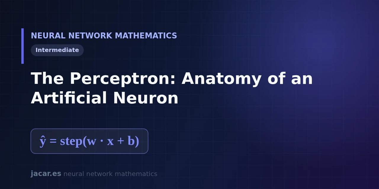
Table of contents
- Key takeaways
- What is a perceptron?
- Inputs, weights and bias
- The activation function
- What it can and cannot learn
- Example: a logic gate
- Frequently asked questions
- How does a perceptron differ from a real neuron?
- Why can a perceptron not learn XOR?
- Is the perceptron still useful today?
- Conclusion
- Sources
The perceptron is the simplest artificial neuron and the starting point of every neural network. It takes some inputs, weights them, adds a bias and decides an output with an activation function. Understanding that mechanism means understanding, in miniature, what a whole network does.
In this guide we open the perceptron piece by piece: what it computes, what it can learn and where its limit lies. The same explanation is available in Spanish.
Key takeaways
- The perceptron is an artificial neuron that combines a vector of inputs into a single binary decision.
- Its computation reduces to
ŷ = step(w · x + b): it weights the inputs, adds the bias and applies an activation function. - Frank Rosenblatt introduced it in 1958; his Mark I machine used 400 photocells in a 20 by 20 grid to "see" patterns.
- A single perceptron only separates data linearly, so it cannot learn the XOR function, as Minsky and Papert proved in 1969.
- Stacking perceptrons in layers overcomes that limit: that is the idea behind the mathematics of neural networks roadmap.
What is a perceptron?
A perceptron is a mathematical model of a neuron: it takes a vector of input numbers and produces a single output number, almost always a 0 or a 1. It is the most basic decision unit in machine learning, and everything else is built on top of it.
Frank Rosenblatt, a psychologist at Cornell’s aeronautical laboratory, introduced it in 1958 in the journal Psychological Review. It was not only theory: he built a physical machine, the Mark I Perceptron, with 400 photocells arranged in a 20 by 20 grid and potentiometers that adjusted the weights automatically. The press of the time greeted it with wild enthusiasm; The New York Times, in 1958, described it as «the embryo of an electronic computer that the Navy expects will be able to walk, talk, see and be conscious of its existence». Reality proved more modest, but the idea was revolutionary: a machine that learns from examples.
Inputs, weights and bias
The perceptron works with three ingredients. The inputs are the data, written as a vector x = (x₁, x₂, …, xₙ). The weights w = (w₁, w₂, …, wₙ) measure how important each input is. The bias b is a number that shifts the decision, like the intercept of a line.
The heart of the computation is the dot product between weights and inputs, the same operation we study in the dot product and the neuron:
$$z = \mathbf{w}\cdot\mathbf{x} + b = \sum_{i} w_i x_i + b = w_1 x_1 + w_2 x_2 + \dots + w_n x_n + b$$
That value z (sometimes called the pre-activation) summarises all the evidence for or against firing the neuron. If weight w₂ is large and positive, input x₂ pushes hard towards "yes"; if it is negative, it pushes towards "no". The bias sets how demanding the neuron is before it decides.
The activation function
The number z is not yet a decision, only a score. The activation function turns it into an output. In the classic perceptron that function is the step function: it returns 1 if z ≥ 0 and 0 otherwise. So the full neuron formula is:
$$\hat{y} = \operatorname{step}(\mathbf{w}\cdot\mathbf{x} + b)$$
You can dig deeper into it in the step function. The step has a problem: its derivative is zero almost everywhere, which makes it impossible to train deep networks with gradient descent. That is why modern networks replace the step with smooth functions such as the sigmoid or ReLU, but the structure activation(weights · inputs + bias) is exactly the same as in 1958.
What it can and cannot learn
A perceptron draws a decision boundary that is a straight line (or a plane, in higher dimensions). Anything on one side is classified as 1 and anything on the other as 0. This works perfectly when the two classes are linearly separable, that is, when a straight line can divide them without errors.
The decision boundary is exactly the set of points where $\mathbf{w}\cdot\mathbf{x} + b = 0$: a straight line in two dimensions and a hyperplane in more. Changing the bias $b$ shifts that boundary without rotating it.
The limit arrived in 1969, when Marvin Minsky and Seymour Papert published Perceptrons and proved that a single perceptron cannot solve the XOR function, because its cases are not separable by a single line. That critique cooled funding and opened the first "AI winter". The solution, which took years to catch on, is to stack neurons in more than one layer: a multilayer network does solve XOR, and with backpropagation it can be trained efficiently.
See why XOR is not separable
XOR is 1 at $(0,1)$ and $(1,0)$, and 0 at $(0,0)$ and $(1,1)$.
A separating line $\mathbf{w}\cdot\mathbf{x} + b = 0$ would need $b<0$ (so $(0,0)$ gives 0), $w_1 + b \geq 0$ and $w_2 + b \geq 0$ (so $(1,0)$ and $(0,1)$ give 1), and $w_1 + w_2 + b < 0$ (so $(1,1)$ gives 0). Adding the two middle inequalities gives $w_1 + w_2 \geq -2b$, while the last one demands $w_1 + w_2 < -b$. Since $b<0$ we have $-2b > -b$, so no value can satisfy both. No such line exists.
Example: a logic gate
Let us look at a perceptron that computes the AND gate, which returns 1 only when both inputs are 1. We pick weights $w_1 = 1$, $w_2 = 1$ and bias $b = -1.5$, and apply the step to $z = x_1 + x_2 – 1.5$:
- Inputs $(0, 0)$: $z = -1.5$, output $\operatorname{step}(-1.5) = 0$.
- Inputs $(1, 0)$: $z = -0.5$, output $0$.
- Inputs $(0, 1)$: $z = -0.5$, output $0$.
- Inputs $(1, 1)$: $z = 0.5$, output $\operatorname{step}(0.5) = 1$.
The neuron reproduces the AND truth table with just three adjustable numbers. If you tried the same with XOR, you would find no trio of weights and bias that works: that is where a single perceptron falls short and a second layer becomes necessary.
Frequently asked questions
How does a perceptron differ from a real neuron?
A perceptron is a mathematical simplification. It borrows the idea that a neuron sums incoming signals and "fires" once a threshold is crossed, but it drops the chemistry, the timing and the biology. It is a useful model, not a copy of the brain.
Why can a perceptron not learn XOR?
Because XOR is not linearly separable: no straight line can keep the cases that give 1 on one side and those that give 0 on the other. A perceptron only draws straight boundaries, so it needs at least one hidden layer to solve it.
Is the perceptron still useful today?
Yes, as a concept. Every neuron in a deep network is a perceptron with a smooth activation function. Understanding the original makes it far easier to grasp models with billions of parameters.
Conclusion
The perceptron condenses the central idea of deep learning into one formula, $\hat{y} = \operatorname{step}(\mathbf{w}\cdot\mathbf{x} + b)$: weight the inputs, add a bias and decide with an activation. Knowing its anatomy and its limit (linear separability) is the best starting point before studying multilayer networks. The natural next step is to review the full mathematics of neural networks roadmap.
Sources: [1] Perceptron (Wikipedia)[1], [2] Deep Learning (Goodfellow, Bengio and Courville)[2], [3] Neural Networks and Deep Learning (Michael Nielsen)[3].