What Mathematics Is Behind Neural Networks
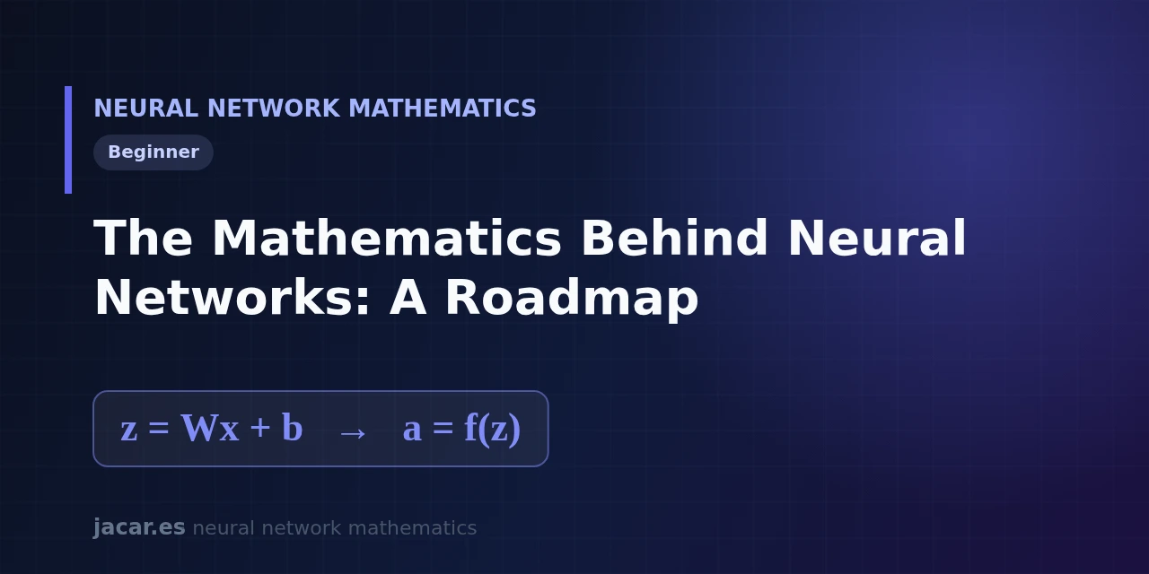
Table of contents
- Key takeaways
- What mathematics does a neural network need
- Linear algebra, the language of data
- Calculus, how the network learns
- Probability and optimisation
- The learning roadmap step by step
- Frequently asked questions
- What level of maths do I need to start?
- Why is the chain rule so important?
- Do I need to code to learn this maths?
- Conclusion
- Sources
Behind every neural network, three branches of mathematics work together. Linear algebra organises the data and the weights, calculus measures how the error changes, and probability decides what counts as a correct answer. Understanding those pieces turns the network from a black box into a system you can reason about.
This guide is the roadmap: what to study, in what order and how each block fits. The same explanation is available in Spanish.
Key takeaways
- The mathematics of neural networks stands on three pillars: linear algebra, calculus and probability.
- Linear algebra represents data, weights and layers as vectors and matrices; a layer is essentially a matrix multiplication.
- Calculus, and specifically the chain rule, is what lets the network learn by adjusting its weights with gradient descent.
- Probability gives meaning to loss functions and to the outputs we read as probabilities.
- A model like GPT-3 tunes 175 billion parameters with these rules: deep learning is that machinery at scale.
What mathematics does a neural network need
A neural network is just a function that takes numbers, combines them and returns other numbers. To build and understand that function you need three tools. The reference book Mathematics for Machine Learning[1] captures exactly that set: linear algebra, geometry, vector calculus, optimisation and probability, and uses it to derive four central machine learning methods.
The good news is that you do not need to be a professional mathematician. With first-year linear algebra, a firm grasp of derivatives and a basic idea of probability, you can follow 90% of what happens inside a network. The rest is practice and repetition.
Linear algebra, the language of data
Every piece of data that enters a network (an image, a sentence, a table row) becomes a vector: an ordered list of numbers. The weights of each layer form a matrix, and computing a layer’s output means multiplying that matrix by the input vector. That is why graphics cards, built to multiply matrices, are the engine of deep learning.
The fundamental operation is the dot product $\mathbf{w} \cdot \mathbf{x}$ between inputs and weights, the same one we study in the sigmoid function and every other neuron. In compact notation, a layer computes:
$$z = \mathbf{W}\mathbf{x} + \mathbf{b}$$
where $\mathbf{W}$ is the weight matrix, $\mathbf{x}$ the input vector and $\mathbf{b}$ the bias.
Calculus, how the network learns
Here comes the part that turns a static network into a learning one. Training means changing the weights little by little to reduce the error. To know which direction to move them we use derivatives: they measure how the error responds to a small change in each weight.
Because a network chains many functions together, the key tool is the chain rule, which shares out responsibility for the error layer by layer. Gradient descent updates each weight as $w \leftarrow w – \eta \cdot \frac{\partial L}{\partial w}$, where $\eta$ is the learning rate and $\frac{\partial L}{\partial w}$ the gradient of the error. That sharing is backpropagation.
The algorithm became popular in 1986 with the paper by Rumelhart, Hinton and Williams in Nature, «Learning representations by back-propagating errors»[2], which showed how to compute the gradient of every weight in a single backward pass. As Geoffrey Hinton put it about that idea, «the brain has to be getting gradients somehow, and backpropagation is the most efficient way we know to do it».
Gradient descent does not search for the global minimum of the error, which is intractable with millions of parameters; it walks down the local slope to a minimum that is good enough. That this works so well in practice is one of the surprises of deep learning.
Probability and optimisation
Probability enters at two moments. First, the outputs of a classification network are read as probabilities: the softmax function turns numbers into a distribution that sums to 1. Second, loss functions such as cross-entropy measure the distance between the prediction and the correct answer using ideas from information theory.
With the loss defined, optimisation is what adjusts the weights. The basic method, gradient descent, takes small steps in the direction that most reduces the error. Frank Rosenblatt’s original perceptron, from 1958, already adjusted weights with a similar, far simpler rule.
The learning roadmap step by step
This is the order we follow in the full route:
- Foundations: vectors, matrices, dot product, derivatives and the chain rule.
- The neuron and forward propagation: weights, biases and activation functions.
- Loss functions: how to measure the error.
- Training: gradient descent and backpropagation.
- Advanced optimisation: momentum, Adam and friends.
- Stability: initialisation, normalisation and regularisation.
Each block builds on the previous one. If something does not click, stepping back one item on the list almost always helps.
Frequently asked questions
What level of maths do I need to start?
Basic linear algebra (vectors and matrices), single- and multi-variable derivatives and an intuitive notion of probability are enough. You do not need advanced analysis or topology to understand and program neural networks.
Why is the chain rule so important?
Because a network is a composition of many functions, and the chain rule is what lets you compute how each weight affects the final error. Without it there would be no backpropagation, and without backpropagation we could not train 175-billion-parameter models like GPT-3.
Do I need to code to learn this maths?
It is not mandatory, but it helps a lot. Implementing a neuron or a layer in code cements the concepts better than any proof, because it forces you to handle the dimensions of vectors and matrices precisely.
Conclusion
The mathematics of neural networks is not a wall but a map of three connected regions: linear algebra to represent, calculus to learn and probability to decide. With that map in mind, every new topic finds its place. The natural next step is to start with the foundations and work up to the softmax function and backpropagation.