The Vanishing Gradient Problem
Table of contents
- Key takeaways
- What the vanishing gradient problem is
- Why sigmoid and hyperbolic tangent cause it
- The mathematics, a product of derivatives smaller than 1
- Solutions (ReLU, initialisation, normalisation)
- Example in a deep network
- Frequently asked questions
- Why is it called the vanishing gradient?
- Does ReLU fully remove the problem?
- Does it affect only deep networks?
- Conclusion
- Sources
The vanishing gradient problem is the reason deep networks failed to learn for years. As the error travels backward layer by layer, it is multiplied by a small derivative at each step and shrinks until it almost disappears. The early layers receive such a weak signal that their weights barely change, and the network stalls.
Understanding why this happens and how to avoid it is central to training deep models. The same explanation is available in Spanish.
Key takeaways
- The vanishing gradient problem appears when the error signal shrinks as it backpropagates layer after layer, and the early layers stop learning.
- The mathematical cause is a product of derivatives smaller than 1: the sigmoid’s peaks at 0.25 and the hyperbolic tangent’s at 1.
- With 10 layers and a derivative of 0.25 in each, the gradient is multiplied by 0.25 ten times and ends up around 0.000001, effectively zero.
- Sepp Hochreiter formalised the problem in 1991, and Bengio, Simard and Frasconi studied it in recurrent networks in 1994.
- The usual fixes are the ReLU activation, careful weight initialisation and batch normalisation.
What the vanishing gradient problem is
A neural network learns by adjusting its weights to reduce the error. To know how much to adjust each one, it computes the gradient: the derivative of the loss with respect to that weight. That computation uses the chain rule, which shares responsibility for the error from output to input. It is the basis of backpropagation, which we covered in the mathematics of neural networks roadmap.
The problem comes from how that sharing works. To reach the gradient of a first-layer weight, you must multiply the derivatives of every layer above it. If those derivatives are smaller than 1, the product gets smaller and smaller as we move back.
In a deep network, the gradient reaching the first layer can be so tiny that the weight does not move, and that layer never learns useful features. That fading is what the hero formula expresses, $\dfrac{\partial L}{\partial w^{(1)}} \to 0$.
Why sigmoid and hyperbolic tangent cause it
Classic activation functions squeeze their input into a narrow range, and that is the trap. The sigmoid function maps any number to the interval between 0 and 1, and its derivative never exceeds 0.25, a value it reaches right at the centre. In the tails, when the neuron is saturated, the derivative approaches 0.
The hyperbolic tangent improves things a little because it is centred at 0 and its derivative reaches 1 at the origin, but it also saturates and drops to 0 at the extremes. With activation $a = f(z)$ and $z = \mathbf{W}x+b$, each layer contributes a factor $f'(z)$ to the gradient. Since those factors are almost always smaller than 1, each added layer multiplies the gradient by another small number, and the result collapses. That is why the problem worsens exactly with depth, which is precisely what gives deep learning its power.
The mathematics, a product of derivatives smaller than 1
$$\frac{\partial L}{\partial w^{(1)}} = \frac{\partial L}{\partial a^{(n)}} \prod_{i=2}^{n} f'(z^{(i)})\,w^{(i)}$$
Let us put numbers on it. Suppose a network with 10 layers where, in each one, the activation derivative equals 0.25, the sigmoid maximum. The gradient reaching the first layer includes the factor $0.25^{10} \approx 0.000001$. In other words, the signal has been reduced to a millionth before it reaches the start of the network.
This decay is geometric, not linear: every layer you add multiplies the gradient by another factor smaller than 1, so the problem grows exponentially with depth.
Show the derivation
By the chain rule, the gradient of a first-layer weight is the product of the derivatives of every layer above it: $\dfrac{\partial L}{\partial w^{(1)}} = \dfrac{\partial L}{\partial a^{(n)}}\prod_{i=2}^{n} f'(z^{(i)})\,w^{(i)}$. If each $f'(z^{(i)}) \le 0.25$, then $\prod_{i=2}^{n} f'(z^{(i)}) \le 0.25^{\,n-1}$, which for $n=11$ gives $0.25^{10} \approx 0.000001$.
If instead of 0.25 we use a smaller, more typical value, the drop is even more brutal. This exponential behaviour is the essence of the phenomenon: the gradient is not just a bit smaller, it decays geometrically with the number of layers. The same mechanism, with derivatives larger than 1, produces the opposite effect, the exploding gradient, which also prevents training. As the work of Bengio and colleagues on recurrent networks puts it, «learning long-term dependencies with gradient descent is difficult» precisely because of this multiplicative dynamic.
Solutions (ReLU, initialisation, normalisation)
The most direct fix was to change the activation function. ReLU returns the value as is if it is positive and 0 if it is negative, so its derivative equals exactly 1 in the active region. Because it does not compress the signal, it does not shrink it, and the gradient propagates without vanishing. It was one of the keys that enabled training deep networks from 2011 onward.
The second piece is weight initialisation. Methods such as Xavier Glorot and Yoshua Bengio’s, or Kaiming He’s, choose the initial scale of the weights so that the variance of the signal stays stable from layer to layer. The third is batch normalisation, which rescales the activations inside the network and makes the optimisation more stable. Combined with residual connections, these techniques are what today allow training networks of hundreds of layers without the gradient dying.
Example in a deep network
Picture a 20-layer network with sigmoids trying to classify images. During training, you measure the magnitude of the gradient at each layer. In the layers near the output the gradients have a reasonable size, but as you move toward the input you see them fall by a factor of ten again and again. By the time you reach layer 1, the gradient is so small that its weights stay almost identical to their initial values, epoch after epoch.
The practical symptom is clear: the loss drops at first and then stalls, and the early layers never learn to detect edges or basic textures. If you replace the sigmoids with ReLU, add batch normalisation and a proper initialisation, the gradients recover a healthy size across all layers and the whole network starts to learn. That contrast is the best proof that the problem is real and that its solutions work.
Frequently asked questions
Why is it called the vanishing gradient?
Because the gradient, the signal that tells you how to adjust each weight, gets smaller and smaller as it backpropagates toward the first layers until it approaches zero. When the gradient is nearly 0, the weight is not updated and the layer stops learning, as if the signal had vanished along the way.
Does ReLU fully remove the problem?
It reduces it a lot because its derivative equals 1 in the positive region, so it does not shrink the gradient. It is not a total fix: the dying-neuron problem can appear when the input is always negative. That is why the standard recipe pairs it with good initialisation, batch normalisation and variants like Leaky ReLU.
Does it affect only deep networks?
It is worse the more layers there are, because more derivatives smaller than 1 are multiplied. It also hits recurrent networks hard, since they unroll one time step per element of the sequence and suffer the same multiplicative effect; that was the reason architectures like LSTM were invented.
Conclusion
The vanishing gradient problem is a multiplication problem: one derivative smaller than 1 per layer makes the error signal arrive almost null at the first layers. Recognising the cause, the functions that saturate, leads naturally to the solution, activations like ReLU, careful initialisation and normalisation. With those tools, depth stops being an obstacle and becomes the advantage that defines deep learning.