
L1 and L2 Regularization (Weight Decay)
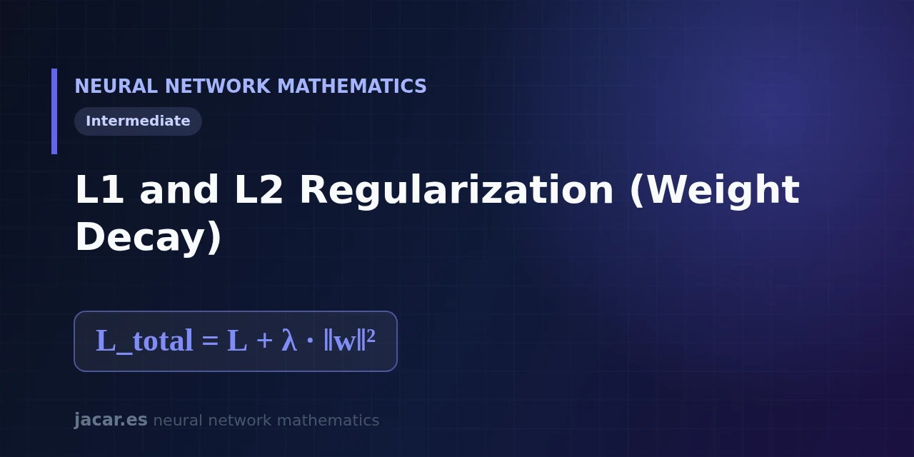
Table of contents
- Key takeaways
- What is regularization?
- L2 regularization (weight decay)
- L1 regularization and sparsity
- The lambda term
- Effect on overfitting
- Frequently asked questions
- What is the difference between L1 and L2 regularization?
- What exactly is weight decay?
- How do I choose the value of lambda?
- Conclusion
- Sources
L1 and L2 regularization is the most direct way to stop a neural network from memorising its training data. The idea: you add an extra term to the loss function that penalises large weights, so the network prefers simple solutions. L2, known as weight decay, shrinks the weights little by little; L1 forces the ones that contribute nothing to be exactly zero.
Understanding both clarifies why one model generalises well while another gets stuck parroting the training set. The same explanation is available in Spanish.
Key takeaways
- L1 L2 regularization changes the loss: instead of minimising the error $L$ alone, the network minimises $L_{\text{total}} = L + \lambda \lVert \mathbf{w} \rVert^2$ (for L2) or $L + \lambda \lVert \mathbf{w} \rVert_1$ (for L1).
- L2 regularization (ridge or weight decay) adds the squared norm of the weights and shrinks them smoothly towards zero without ever nulling them.
- L1 regularization (lasso) adds the absolute value of the weights and tends to set them exactly to zero, producing sparse models and selecting features.
- The coefficient $\lambda$ (lambda) controls the strength of the penalty: typical values run from 0.00001 to 0.1, tuned by cross-validation.
- Both techniques reduce overfitting by curbing the model’s variance, at the cost of a small increase in bias.
What is regularization?
Regularizing is any change we make to a model with the goal of reducing its generalisation error without necessarily reducing its training error. Put another way, we want the network to be right on data it has never seen, not only on data it already knows.
Overfitting appears when the network has so much freedom that it learns even the noise in the training examples. A typical sign is that the training error drops to almost 0 while the validation error starts to climb.
The most common regularization in neural networks attacks that problem through the weights: it adds to the loss a term that grows when the weights grow. So the formula the network tries to minimise stops being just $L$ and becomes $L_{\text{total}} = L + \lambda R(\mathbf{w})$, where $R(\mathbf{w})$ measures the size of the weights. The reference text Deep Learning[1] devotes its whole chapter 7 to these strategies.
L2 regularization (weight decay)
L2 regularization uses the squared L2 norm of the weights as the penalty: $R(\mathbf{w}) = \lVert \mathbf{w} \rVert^2 = \sum_i wi^2$. The full loss becomes $L{\text{total}} = L + \lambda \sum_i w_i^2$, which is exactly the formula in this article’s hero.
Its nickname, weight decay, comes from the effect it produces during training. Differentiating the term $\lambda \sum_i w_i^2$ gives a gradient $2\lambda w$, and the descent step subtracts $\eta \cdot 2\lambda w$ from every weight at each update. In practice, each weight is multiplied by a factor slightly below 1 before the error gradient is applied, so it decays towards zero continuously.
This variant is also known as ridge regression or Tikhonov regularization, and Krogh and Hertz showed back in 1991 that this simple decay improves generalisation. Almost every modern optimizer ships it built in: in PyTorch it is the weight_decay argument and in scikit-learn[2] it is the Ridge class. Because it penalises large values more, it spreads the weight across more connections rather than concentrating it in a few.
Show the derivation
Start from the penalty $R(\mathbf{w}) = \sum_i w_i^2$. Its gradient with respect to a weight is $\dfrac{\partial R}{\partial w_i} = 2 w_i$, so the gradient of the full term is $\nabla_{\mathbf{w}}\,\lambda R = 2\lambda\mathbf{w}$. The descent step with learning rate $\eta$ updates $w_i \leftarrow w_i-\eta(\partial L/\partial w_i)-\eta\,2\lambda w_i = (1-2\eta\lambda)\,w_i-\eta\,\partial L/\partial w_i$. The factor $(1-2\eta\lambda)$, slightly below 1, is what shrinks each weight at every update: that is weight decay.
L1 regularization and sparsity
L1 regularization swaps the penalty for the sum of absolute values: $R(\mathbf{w}) = \lVert \mathbf{w} \rVert_1 = \sum_i |wi|$. The loss becomes $L{\text{total}} = L + \lambda \sum_i |w_i|$, and that seemingly small difference changes the outcome a lot.
The key is in the gradient: L2 pushes each weight with a force proportional to its value ($2\lambda w$), which fades near zero, whereas L1 pushes with a constant force ($\pm\lambda$) that never eases off. That is why L1 can pin weights at exact zero and L2 cannot.
The reason lies in the gradient. The derivative of the absolute value is constant (it is $+\lambda$ or $-\lambda$ depending on the weight’s sign). L1 therefore pushes each weight towards zero with the same force no matter how small it already is.
L2, by contrast, pushes with a force proportional to the weight, which weakens as the weight approaches zero. The result is that L1 leaves weights at exact zero, producing a sparse model where only the useful connections survive.
This variant is called lasso. As Goodfellow, Bengio and Courville put it in Deep Learning[1], «in comparison to L2 regularization, L1 regularization results in a solution that is more sparse». That sparsity makes L1 a feature-selection tool: it discards whole inputs by setting their weight to zero.
The lambda term
The coefficient $\lambda$ is a hyperparameter that decides how much the penalty weighs against the original error. With $\lambda = 0$ there is no regularization and the network can overfit unchecked; with a large $\lambda$, the penalty term dominates and all weights get so close to zero that the network loses capacity and underfits.
The balance sits in an intermediate range. On real problems, $\lambda$ ranges from 0.00001 to 0.1, and multiplying its value by 10 has a noticeable effect, so it is explored on a logarithmic scale. There is no universal value: you pick it by trying a grid of candidates and measuring the validation error, normally with 5- or 10-fold cross-validation. Watch out for the naming, because each library uses its own: in scikit-learn the argument is called alpha, while in logistic regression it is controlled by C, which equals $1/\lambda$, so a small C means strong regularization.
Effect on overfitting
Behind all this is the bias-variance trade-off. An unregularized model has low bias but high variance: it fits each sample too closely and changes a lot from one dataset to another. By penalising large weights, regularization lowers that variance and smooths the function the network represents, in exchange for adding a little bias. The sweet spot minimises the sum of the two.
In practice this shows up as a smaller gap between the training and validation errors. If a network reaches 99% accuracy in training and only 80% in validation, those 19 points of difference are the classic signature of overfitting, and raising $\lambda$ is what narrows that gap. When you want to combine the best of both techniques you use the elastic net, which adds an L1 term and an L2 term with their own coefficients. All of this fits inside the wider map that walks through the mathematics of neural networks.
Frequently asked questions
What is the difference between L1 and L2 regularization?
L1 penalises the sum of the absolute values of the weights and tends to set them to exact zero, giving sparse models and serving as feature selection. L2 penalises the sum of squares and shrinks the weights smoothly without nulling them, spreading importance over the whole set of connections. In short, L1 selects and L2 moderates.
What exactly is weight decay?
It is another name for L2 regularization seen from the training side. Because the gradient of the term $\lambda \lVert \mathbf{w} \rVert^2$ is proportional to the weight, each update multiplies the weight by a factor slightly below 1 before applying the error gradient. That continuous shrinking towards zero is what is called weight decay, and it is the weight_decay argument of most optimizers.
How do I choose the value of lambda?
There is no single value. You try a grid of candidates on a logarithmic scale, for example 0.0001, 0.001, 0.01 and 0.1. Keep the one that gives the lowest validation error. Cross-validation with 5 or 10 folds is the standard method for making that comparison reliably.
Conclusion
L1 and L2 regularization does not change the network’s architecture, only the goal it pursues: instead of driving the error down at any cost, it seeks the lowest error achievable with small weights. L2 shrinks them smoothly and spreads the work; L1 clips them to zero and leaves a sparse model; the coefficient $\lambda$ sets the dose. With those three ideas you understand why almost no serious training goes without regularization. The natural next step is to review the vector norms L1 and L2, which are the geometric basis of all this.