Layer Normalization and Variants
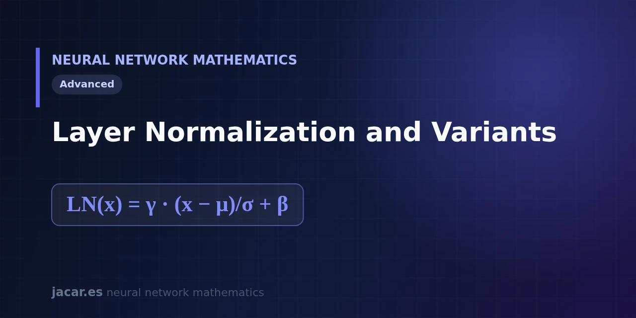
Table of contents
- Key takeaways
- What layer normalization is
- Layer norm versus batch norm
- Why transformers rely on it
- RMSNorm and other variants
- Where it goes: pre-norm and post-norm
- Frequently asked questions
- What is the difference between layer norm and batch norm?
- Why do transformers use layer normalization?
- Is it worth switching to RMSNorm?
- Conclusion
- Sources
Layer normalization is the technique that keeps a transformer’s training stable by normalizing each example on its own. Instead of looking at the whole batch, it computes the mean and standard deviation over the features of a single sample and rescales those values. That independence from batch size is why almost every large language model uses it.
Here you will see what it does, how it differs from batch normalization and why RMSNorm has replaced it in practice. The same explanation is available in Spanish.
Key takeaways
- Layer normalization normalizes a single example’s activations across its features: $\mathrm{LN}(x) = \gamma \cdot (x-\mu)/\sigma + \beta$, with $\mu$ and $\sigma$ computed per sample.
- Because it does not depend on the batch, it behaves the same in training and inference and tolerates a batch size of 1, which batch normalization cannot.
- Transformers, introduced in 2017, adopted it because sequence lengths vary and batch statistics would be unstable.
- RMSNorm (2019) drops the mean centering and only rescales by the root mean square, saving between 7% and 64% of the running time.
- Placement matters: pre-normalization stabilizes deep networks better than the original post-normalization.
What layer normalization is
Proposed by Ba, Kiros and Hinton in 2016, layer normalization takes a layer’s activation vector for one example, $z = \mathbf{W}x + b$, and rescales it to have zero mean and unit variance. It then applies two learnable parameters, a gain $\gamma$ and a shift $\beta$, that give the network back the freedom to adjust the scale.
The compact formula is:
$$\mathrm{LN}(x) = \gamma \cdot \dfrac{x-\mu}{\sigma} + \beta$$
where $\mu$ is the mean of that example’s activations, $\sigma$ its standard deviation, and a small $\varepsilon$ sits under the root to avoid dividing by zero. The key is the axis of the computation: $\mu$ and $\sigma$ run over the features of a single sample, not the batch dimension. To review where those activations come from, revisit the mathematics behind neural networks roadmap.
The small $\varepsilon$ added under the root does not change the scale: it only prevents division by zero when an example’s variance is tiny. In PyTorch its default value is $\varepsilon = 10^{-5}$.
In pseudocode, the per-token operation fits in three lines:
mu = x.mean(-1, keepdim=True)          # mean over the features
var = x.var(-1, keepdim=True, unbiased=False)
y = gamma * (x - mu) / (var + eps).sqrt() + beta
Layer norm versus batch norm
Batch normalization, by Ioffe and Szegedy (2015), normalizes each feature using the mean and variance computed over the whole batch. That ties it to the batch size and composition, and forces it to keep running statistics for inference. Layer normalization flips that axis: it normalizes each example over its own features, so it needs no global statistics and no separate test-time mode.
The practical consequences are three. First, it works with small batches or a batch size of 1, typical in long sequences. Second, the computation is identical in training and inference. Third, it introduces no dependency between examples in the same batch, which simplifies parallelism.
The original description puts it this way: layer normalization computes the mean and variance «from all of the summed inputs to the neurons in a layer on a single training case».
Why transformers rely on it
In a transformer, the sequence length changes from one example to the next and attention mixes tokens within each sample. A batch statistic would be noisy and unstable, whereas normalizing per token is clean and deterministic. That is why the 2017 paper that introduced the architecture placed a layer normalization after each sublayer, and every model in the GPT family inherited it.
A model like GPT-3 stacks 96 such layers, and without robust normalization that depth would be hard to train. The same idea appears in the step before the softmax function of the output layer.
RMSNorm and other variants
RMSNorm, by Zhang and Sennrich (2019), starts from a simple observation: perhaps the mean centering adds little. Its variant removes the subtraction of $\mu$ and only divides by the root mean square of the activations, keeping the gain $\gamma$. As the authors summarize, «the re-centering invariance in LayerNorm is dispensable».
The benefit is purely efficiency: by skipping the mean computation, RMSNorm cuts running time by between 7% and 64% depending on the model, with no measurable loss of quality. That advantage explains why LLaMA, T5 and much of today’s open models use it by default. Other variants tweak where and how the scaling happens, but they share the same root as the sigmoid function and the rest of the toolkit: rescaling activations to keep gradients in a healthy range.
Where it goes: pre-norm and post-norm
The position of the normalization relative to the residual connection defines two styles. In post-normalization, the original transformer’s choice, the layer is applied after adding the residual. In pre-normalization it is applied inside the branch, before the sublayer. Xiong and colleagues showed in 2020 that pre-normalization keeps gradients well bounded from initialization, while post-normalization needs a learning-rate warmup of $\eta$ to avoid diverging.
That is why modern deep models, including GPT-2 and GPT-3, went for pre-normalization: it allows larger learning rates and more reliable convergence. The rule of thumb is clear: the more layers you stack, the more you want to normalize before the sublayer.
Frequently asked questions
What is the difference between layer norm and batch norm?
Batch normalization computes the mean and variance over the batch dimension, one value per feature, and depends on the batch size. Layer normalization computes them over the features of a single example, so it needs no global statistics and no different behavior at inference time.
Why do transformers use layer normalization?
Because sequences have variable lengths and batch statistics would be unstable. Normalizing each token over its own features is deterministic and works with any batch size, including 1, which fits both training and text generation.
Is it worth switching to RMSNorm?
In large models, almost always yes. RMSNorm delivers the same quality as layer normalization while saving between 7% and 64% of compute. That is why it is the default in recent open models like LLaMA.
Conclusion
Layer normalization solved the problem of stabilizing networks whose batch statistics are unreliable, and in doing so made deep transformers feasible. Its natural evolution, RMSNorm, keeps the essential idea and trims the cost. The next step is to understand how this normalization interacts with backpropagation and with batch normalization across other architectures.