Mathematical Formulation of Artificial Neural Network Input
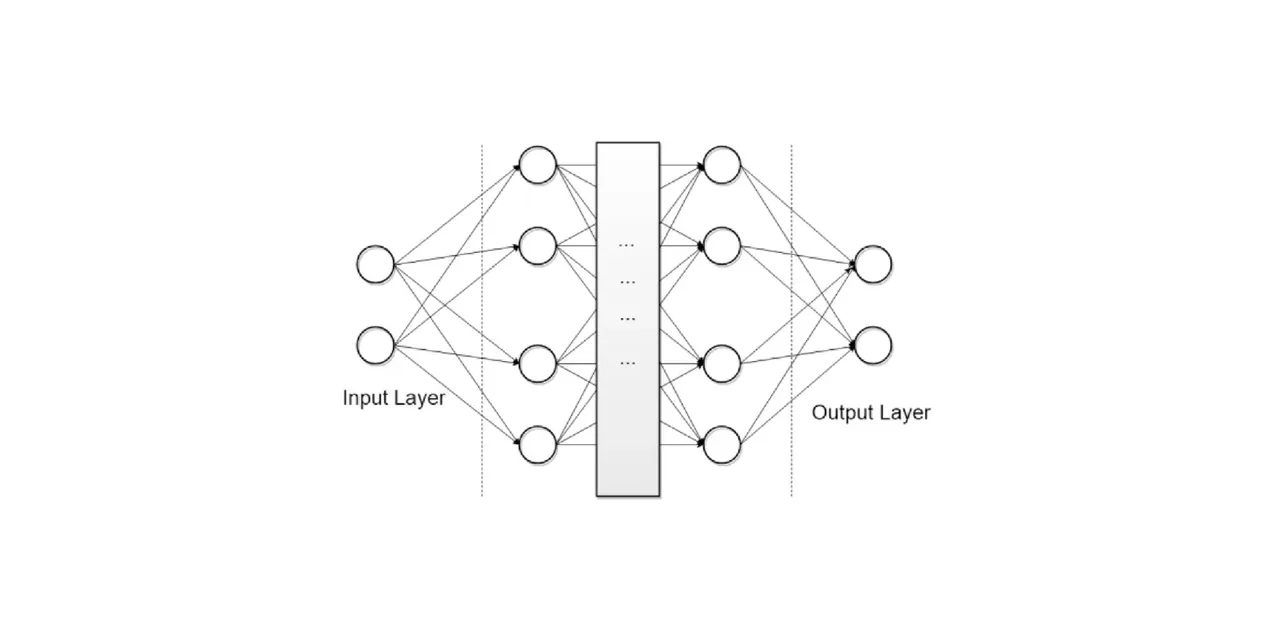
Table of contents
- Key takeaways
- The mathematical representation of the input
- The hidden layer: linear transformation followed by non-linearity
- Activation functions: why they matter
- The backpropagation algorithm
- Conclusion
- Frequently asked questions
- What happens if I build a neural network without an activation function?
- Why does the sigmoid cause vanishing gradients in deep networks?
- What is the bias vector b for in a hidden layer?
Beneath the surface of any neural network lies linear algebra: vectors, matrices, and functions. Understanding the mathematical formulation of the input is not an academic exercise: it is the foundation for debugging models, diagnosing gradient problems, and choosing activation functions with sound reasoning.
Key takeaways
-
Each input to a neural network is represented as a column vector x of n dimensions.
-
The hidden layer applies a linear transformation via a weight matrix W and bias vector b, followed by a non-linear activation function.
-
The activation function introduces non-linearity without which the network would be equivalent to a simple linear regression.
-
Training adjusts weights W and b by minimising a loss function via gradient descent with backpropagation.
-
Vanishing and exploding gradients are the main mathematical problem in deep networks.
The mathematical representation of the input
A data input sample is represented as a column vector of dimension n:
$$mathbf{x} = begin{pmatrix} x_1 x_2 vdots x_n end{pmatrix} in mathbb{R}^n$$
Where each xᵢ is a feature of the data point: a pixel in an image, an encoded word in text, a numerical value in a table. For a batch of B samples, the input is organised as a matrix X of dimension B × n, enabling parallel processing of multiple samples via efficient matrix operations on GPU.
The hidden layer: linear transformation followed by non-linearity
For a hidden layer with M neurons, the operation is:
z = W**x + b**
h = f(z)
Where:
-
W is the weight matrix of dimension M × n. Row j of W contains the weights for neuron j.
-
b is the bias vector of dimension M, which allows shifting the activation independently of the input.
-
f is the activation function, applied element-wise.
The bias b is critical: without it, if all inputs are zero, the output would also be zero regardless of the weights, limiting the network’s expressive capacity.
Activation functions: why they matter
Without a non-linear activation function, the composition of linear layers remains linear. A 100-layer network without activations is mathematically equivalent to a single linear layer. The most commonly used activation functions are:
-
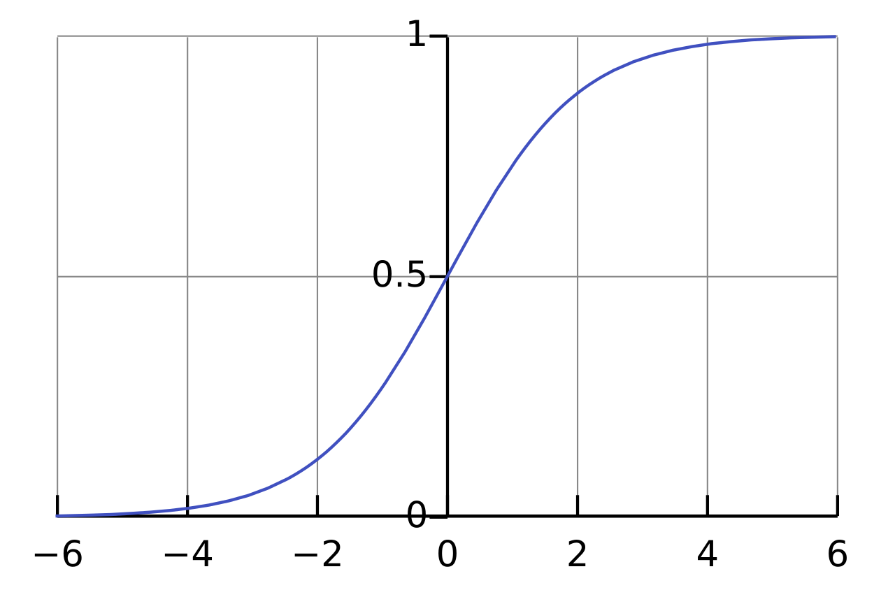
Sigmoid: f(z) = 1 / (1 + e⁻ᶻ), with output in (0,1); useful in the output layer for binary classification, but prone to vanishing gradients in deep networks.
-
ReLU (Rectified Linear Unit): f(z) = max(0, z), computationally efficient and mitigates the vanishing gradient problem; the default function in hidden layers of deep networks.
-
Tanh: f(z) = (eᶻ − e⁻ᶻ) / (eᶻ + e⁻ᶻ), with zero-centred output and better behaviour than sigmoid in hidden layers.
-
Softmax: used in the output layer for multi-class classification; converts a vector of arbitrary values into a probability distribution. See Softmax function.
-
Linear function: f(z) = z, with no transformation; used in the output layer for regression. See linear activation function.
The backpropagation algorithm
Training consists of adjusting W and b to minimise a loss function L (e.g., cross-entropy for classification, MSE for regression). The backpropagation algorithm computes the gradient of L with respect to each parameter using the chain rule:
$$frac{partial L}{partial mathbf{W}^{(l)}} = frac{partial L}{partial mathbf{h}^{(l)}} cdot frac{partial mathbf{h}^{(l)}}{partial mathbf{z}^{(l)}} cdot frac{partial mathbf{z}^{(l)}}{partial mathbf{W}^{(l)}}$$
The process, step by step:
-
Forward pass: compute the network’s prediction.
-
Loss calculation: compare prediction to real label.
-
Backward pass: compute gradients layer by layer from output to input.
-
Parameter update: with gradient descent, W ← W − η · ∂L/∂W, where η is the learning rate.
The vanishing gradient problem occurs when gradients become exponentially small as they propagate backwards layer after layer, mainly with sigmoid and tanh. ReLU and its variants (Leaky ReLU, ELU) mitigate this problem. The opposite problem, exploding gradients, is addressed with gradient clipping.
For more architectural context, see neural networks and deep learning. For multi-class classification from the output layer perspective, see Softmax function. Practical use of these models in rapid benchmarks is covered in LazyPredict in Python.
Conclusion
The mathematical formulation of a neural network is elegant in its structure: linear algebra in each layer, non-linearity in each activation, and iterative optimisation in training. Understanding these fundamentals is not optional for anyone who wants to go beyond using libraries as black boxes. Diagnosing a model that does not converge, choosing the correct activation function, or designing the right architecture all depend directly on understanding the mathematics underneath.
Frequently asked questions
What happens if I build a neural network without an activation function?
The composition of linear layers remains linear: a 100-layer network without activations is mathematically equivalent to a single linear layer, that is, to a simple linear regression. The activation function, applied element-wise to z = Wx + b, is what introduces the non-linearity that gives the network its expressive capacity. That is why ReLU, f(z) = max(0, z), is the default choice in the hidden layers of deep networks.
Why does the sigmoid cause vanishing gradients in deep networks?
Because as the gradient propagates backwards layer after layer via the chain rule, gradients become exponentially small, which happens mainly with sigmoid and tanh. ReLU and its variants (Leaky ReLU, ELU) mitigate this problem, which is why sigmoid is reserved for the output layer in binary classification. The opposite problem, exploding gradients, is addressed with gradient clipping.
What is the bias vector b for in a hidden layer?
It allows shifting the activation independently of the input. Without it, if all inputs are zero the output would also be zero regardless of the weights, limiting the network's expressive capacity. In a layer with M neurons, b has dimension M and accompanies the M × n weight matrix W in the transformation z = Wx + b, before the activation function is applied.