AdaGrad and RMSProp: Adaptive Learning Rates
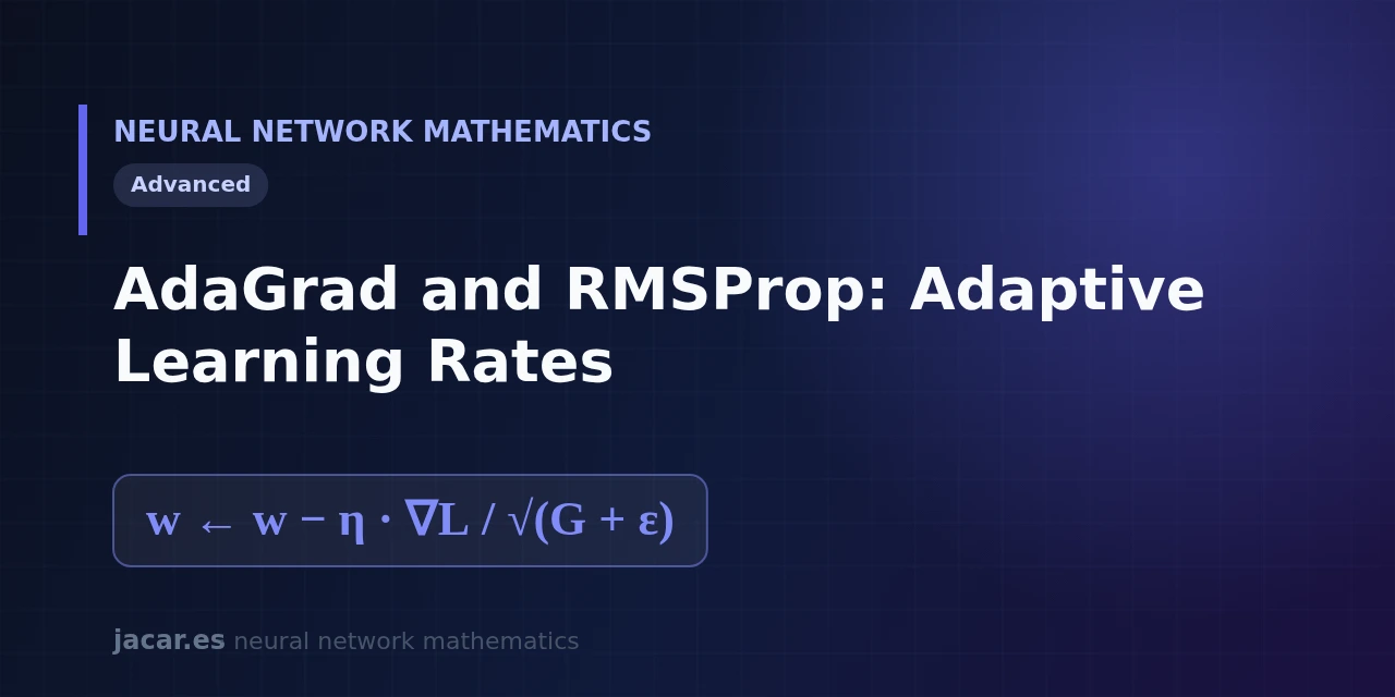
Table of contents
- Key takeaways
- The problem with a single rate
- AdaGrad, accumulating the squared gradient
- AdaGrad's decay
- RMSProp, the moving average
- AdaGrad versus RMSProp
- Frequently asked questions
- What is the main difference between AdaGrad and RMSProp?
- When should I use AdaGrad instead of RMSProp?
- What is the epsilon term in the formula for?
- Conclusion
- Sources
AdaGrad and RMSProp change one simple idea about training: instead of a single learning rate for the whole network, they give every weight its own. AdaGrad shares out that pace according to how much each parameter has moved historically, but it ends up slowing down too much. RMSProp fixes exactly that flaw with a moving average that forgets the distant past.
This guide explains how both work, why they are so alike and when to pick each one. It is part of the mathematics behind neural networks roadmap, and the same explanation is available in Spanish.
Key takeaways
- AdaGrad and RMSProp are adaptive optimisers: each weight $w$ gets its own effective learning rate instead of sharing one global $\eta$.
- AdaGrad accumulates the square of every gradient in a term $G$ and divides the step by $\sqrt{G+\varepsilon}$, with $\varepsilon \approx 10^{-8}$ to avoid dividing by zero.
- AdaGrad’s flaw is that $G$ only ever grows, so the effective rate tends to zero and training stalls too early.
- RMSProp replaces that infinite sum with an exponential moving average using a typical decay factor of $0.9$, which discards the distant past.
- AdaGrad (2011) shines on sparse data; RMSProp (2012) works better in deep networks and is the direct basis of the Adam optimiser.
The problem with a single rate
In classic gradient descent all weights share the same learning rate $\eta$, following the rule $w \leftarrow w-\eta\cdot\nabla L$. The trouble is that not every weight needs the same treatment. Some parameters receive large, frequent gradients; others, tied to features that appear rarely, are almost never updated.
With a single η you have to pick a compromise value. Raise it so the rare weights learn something and the frequent ones destabilise; lower it to tame the frequent ones and the rare ones take forever. The idea of adaptive rates is to break that compromise: take a large step where the signal has been scarce and a small step where it has already been abundant. Formally, the step scale stops being one number and becomes a vector with one value per parameter.
AdaGrad, accumulating the squared gradient
AdaGrad (Adaptive Gradient) was proposed by John Duchi, Elad Hazan and Yoram Singer in 2011, in a Journal of Machine Learning Research paper[1]. Its mechanism is direct: for each weight it keeps an accumulator $G$ that sums the square of every gradient it has received so far. The update becomes $w \leftarrow w-\eta\cdot\dfrac{\nabla L}{\sqrt{G+\varepsilon}}$.
The consequence is elegant. A weight that has seen large gradients has a large $G$, so its denominator grows and its steps shrink. A weight with small gradients keeps a small $G$ and holds on to wide steps.
In practice this shares out the learning rate automatically and makes AdaGrad excel on problems with sparse data, such as text processing, where each feature appears in very few examples. The $\varepsilon$ term, a tiny value on the order of $10^{-8}$, is only there to avoid division by zero on the first step.
AdaGrad’s decay
AdaGrad’s weakness is the sum that makes it work. Because $G$ accumulates squares, which are always positive, it never stops growing. Iteration after iteration the denominator $\sqrt{G+\varepsilon}$ gets bigger, and the effective learning rate $\eta/\sqrt{G+\varepsilon}$ shrinks monotonically toward zero. After thousands of steps the network barely moves even when it still has plenty left to learn.
AdaGrad’s effective rate, $\eta/\sqrt{G+\varepsilon}$, can only decrease: because $G$ never shrinks, each weight’s step gets irreversibly shorter. That is exactly the behaviour RMSProp’s moving average avoids.
This premature shutdown is especially harmful in deep networks, which need far more iterations than the linear models AdaGrad was designed for. Sebastian Ruder puts it clearly in his overview of optimisers: «RMSprop and Adadelta have both been developed independently around the same time stemming from the need to resolve Adagrad’s radically diminishing learning rates», as he explains in his synthesis of optimisation methods[2]. That is exactly the gap RMSProp came to fill.
Show the derivation
After $t$ steps, AdaGrad accumulates $G_t=\sum_{i=1}^{t}(\nabla L_i)^2$. Since every term is non-negative, the sequence $G_t$ is monotonically increasing, so $\sqrt{G_t+\varepsilon}$ grows too and the effective rate $\eta/\sqrt{G_t+\varepsilon}$ decreases monotonically. If the gradients do not vanish, $G_t\to\infty$ and the effective rate tends to $0$. RMSProp replaces the sum with $G_t=\rho G_{t-1}+(1-\rho)(\nabla L_t)^2$; at steady state $G$ settles around the recent mean of $(\nabla L)^2$, so the effective rate does not collapse.
RMSProp, the moving average
RMSProp (Root Mean Square Propagation) was introduced by Geoffrey Hinton in 2012, not in a formal paper but in lecture 6e of his Coursera course on neural networks; his slides remain the original reference[3]. The fix is a single line: instead of summing the squares forever, RMSProp keeps an exponential moving average of them.
At each step it updates the accumulator with $G \leftarrow \rho\cdot G+(1-\rho)\cdot(\nabla L)^2$, where $\rho$ is a decay factor, almost always set to $0.9$. That $\rho$ makes old gradients lose weight gradually: the recent past dominates and the distant past is forgotten. The weight update rule is identical to AdaGrad’s, $w \leftarrow w-\eta\cdot\dfrac{\nabla L}{\sqrt{G+\varepsilon}}$, but now $G$ no longer grows without bound and instead reflects the recent magnitude of the gradient. With that, the effective rate stabilises rather than fading away, and training can continue for as many iterations as needed.
AdaGrad versus RMSProp
The difference between the two fits in a single word: memory. AdaGrad has infinite memory, it remembers every gradient with equal weight and therefore slows down. RMSProp has short memory, controlled by ρ, and therefore stays alive.
In practice this defines when to use each. AdaGrad is still a solid choice for convex models and sparse data, where its braking even helps convergence. RMSProp is the usual pick in deep networks, where the number of iterations is high and AdaGrad’s shutdown would be fatal.
Neither is the end of the road. RMSProp’s moving-average idea was combined with gradient momentum to produce Adam, today the default optimiser in most frameworks. You can widen the context in the Wikipedia entry on stochastic gradient descent[4], which collects AdaGrad, RMSProp and their descendants in one family.
Frequently asked questions
What is the main difference between AdaGrad and RMSProp?
AdaGrad sums the square of every past gradient, so its accumulator only grows and the effective learning rate ends up tending to zero. RMSProp uses an exponential moving average with a decay factor of $0.9$, which forgets old gradients and keeps the rate stable throughout training.
When should I use AdaGrad instead of RMSProp?
AdaGrad performs well on convex problems and sparse data, such as text models where each feature appears in few examples, because its gradual braking is not an obstacle. In deep neural networks, with thousands of iterations, that same braking halts learning, and then RMSProp or Adam are better choices.
What is the epsilon term in the formula for?
The $\varepsilon$ term, a small value on the order of $10^{-8}$, is added inside the root to avoid dividing by zero when the accumulator $G$ is still zero. That happens on the first step or for weights that have not yet received a gradient. It does not change the optimiser’s behaviour, it only keeps the operation numerically stable.
Conclusion
AdaGrad and RMSProp share the same ambition: to give each weight its own learning rate based on its gradient history. AdaGrad achieves it by accumulating squares, but pays the price of slowing to a stop. RMSProp swaps that infinite sum for a moving average with a $0.9$ decay and so keeps a steady pace. Understanding this pair is the best bridge to Adam, which inherits the best of RMSProp and adds gradient momentum.
Sources: [1] Adaptive Subgradient Methods (Duchi, Hazan and Singer, JMLR 2011)[1], [2] An overview of gradient descent optimization algorithms (Sebastian Ruder)[2], [3] Neural Networks for Machine Learning, Lecture 6 (Geoffrey Hinton)[3], [4] Stochastic gradient descent (Wikipedia)[4].