Partial Derivatives and the Gradient in Neural Networks
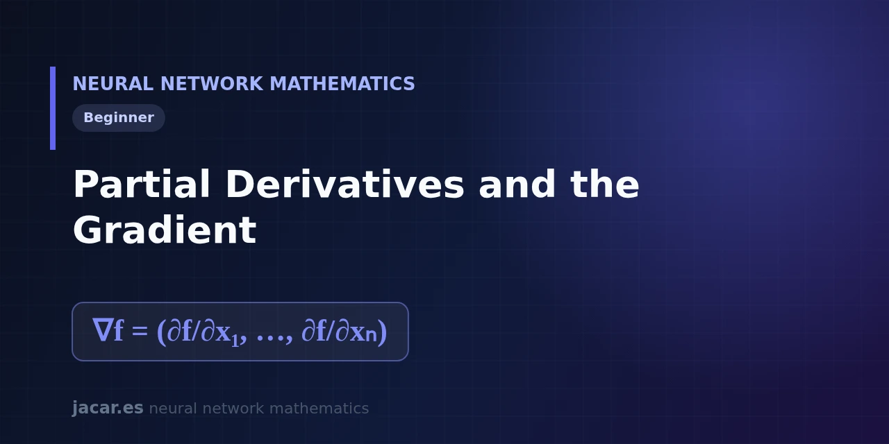
Table of contents
- Key takeaways
- Partial derivatives
- The gradient vector
- What direction the gradient points
- Gradient of a multivariable function
- A worked numerical example
- Frequently asked questions
- How is a partial derivative different from a normal derivative?
- Why does the gradient point to the steepest ascent and not the descent?
- How is the gradient related to training a network?
- Conclusion
- Sources
A partial derivative measures how a function changes when we move a single variable, and the gradient gathers all those derivatives into a vector that shows where the function grows fastest. In a neural network that vector is the compass of training: the error depends on thousands of weights at once, and the gradient tells us how to adjust them all together. This guide explains what a partial derivative is, how the gradient is built and why it points in the direction of steepest ascent. The same explanation is available in Spanish.
Key takeaways
- A partial derivative measures how a multivariable function changes when we alter only one variable and hold the others fixed.
- The gradient is the vector that gathers every partial derivative: $\nabla f = \left(\frac{\partial f}{\partial x_1}, \dots, \frac{\partial f}{\partial x_n}\right)$.
- The gradient points in the direction of steepest ascent; its opposite, the steepest descent, is what training uses.
- In a network the error $L$ depends on all the weights $W$ at once, so we need a partial derivative for each weight, not a single derivative.
- With a small learning rate $\eta$, subtracting the gradient lowers the loss: in the final example it drops from 25 to 16 in one iteration.
Partial derivatives
When a function depends on a single variable, its derivative measures the slope at each point, the rate of change we already covered in derivatives, the rate of change. The problem is that a network’s loss does not depend on one number but on millions of weights.
That is where the partial derivative comes in. The idea: to differentiate with respect to one variable, we treat all the others as constants. If $f(x,y)=x^2+y^2$, the partial derivative with respect to $x$ is $\frac{\partial f}{\partial x}=2x$ (the $y$ is frozen and its term vanishes), and with respect to $y$ it is $\frac{\partial f}{\partial y}=2y$. Each partial answers a local question: if I move this variable a little and touch nothing else, how much and in which direction does the output change?
The symbol $\partial$ (a rounded "d") distinguishes the partial derivative from the ordinary $d$. On Khan Academy[1] you can see the geometric reading: each partial is the slope of the surface along one axis.
The gradient vector
If we compute the partial derivative with respect to each variable and stack them into a list, we get the gradient. For a function of $n$ variables it is written like this:
$$\nabla f = \left(\frac{\partial f}{\partial x_1}, \frac{\partial f}{\partial x_2}, \dots, \frac{\partial f}{\partial x_n}\right)$$
The $\nabla$ symbol is called nabla. The gradient is not a number: it is a vector with as many components as the function has variables. In our example $f(x,y)=x^2+y^2$, the gradient is $\nabla f=(2x,2y)$, a two-component vector that changes at every point of the plane.
Show the derivation
For $f(x,y)=x^2+y^2$ we differentiate with respect to $x$ while treating $y$ as a constant: $\frac{\partial f}{\partial x}=2x$, because the $y^2$ term is constant and its derivative is $0$. Likewise, with respect to $y$: $\frac{\partial f}{\partial y}=2y$. Stacking both partials gives $\nabla f=(2x,2y)$.
This is the missing piece for training networks. Because the error $L$ depends on every weight $W$ in every layer, its gradient has one component per weight. In a real model that means a vector with millions of components, one per parameter. Computing it all efficiently is exactly what backpropagation solves, resting on the chain rule.
What direction the gradient points
Here is the property that makes it so useful: the gradient points in the direction where the function grows fastest, the steepest ascent. Its length tells you how fast it grows. If you are on a hillside and want to climb the steepest path, the gradient marks that direction; if you want to go down, you take the opposite one.
Training wants to lower the error, so it moves in the direction of the negative gradient. As Goodfellow, Bengio and Courville put it in «Deep Learning», «we can decrease f by moving in the direction of the negative gradient». That idea is gradient descent, and the update rule for each weight is $W \leftarrow W-\eta\cdot\nabla L$, where $\eta$ is the learning rate. The method dates back to 1847, when Augustin-Louis Cauchy proposed it to solve systems of equations, long before neural networks existed.
The minus sign in the update rule is what turns ascent into descent: because the gradient $\nabla L$ points toward where the error grows fastest, subtracting it moves the weights exactly toward where the error falls.
One important detail: the gradient only describes the slope right at the point where you stand. That is why training advances in small steps and recomputes the gradient at each one, rather than taking a single long jump.
Gradient of a multivariable function
Let us generalise. A network layer computes $z=Wx+b$ and then an activation $a=f(z)$; by chaining layers, the final loss $L$ becomes a function of all the weights. Its gradient with respect to the weights of layer $l$ is written $\nabla_W L$, and it holds one partial derivative for each entry of the matrix $W$.
The key point is that nothing is new compared with the two-variable case: there are more components. Each partial derivative is computed by freezing the other weights, and the chain rule lets us obtain them all in a single backward pass. That is why a graphics card, which multiplies matrices in parallel, can compute the gradient of millions of parameters in milliseconds. The Wikipedia article on the gradient[2] formalises this generalisation to any number of dimensions.
A worked numerical example
Take $f(x,y)=x^2+y^2$, a bowl-shaped surface whose minimum sits at the origin. We want to reach the bottom starting from the point $(3,4)$.
First, the gradient is $\nabla f=(2x,2y)$. At the point $(3,4)$ that gives the vector $(6,8)$, whose length is 10. That vector points up and outward, away from the minimum, exactly as we expect from the steepest ascent.
To go down, we take a step in the opposite direction with $\eta=0.1$:
$$(x,y)\leftarrow(3,4)-0.1\cdot(6,8)=(2.4,\ 3.2)$$
Let us check that it worked. The initial loss was $f(3,4)=9+16=25$. After the step, $f(2.4,\ 3.2)=5.76+10.24=16$. The loss has dropped from 25 to 16 in a single iteration, having computed only two partial derivatives.
Repeating the process brings the point ever closer to the minimum. That loop, scaled up to millions of weights, is exactly what happens inside a network during training.
Frequently asked questions
How is a partial derivative different from a normal derivative?
The normal derivative applies to functions of a single variable and measures their slope. The partial derivative is used when there are several variables: it differentiates with respect to one and treats the others as constants. A function of three variables has three partial derivatives, one per axis.
Why does the gradient point to the steepest ascent and not the descent?
It is a mathematical property of the vector itself: among all possible directions, the gradient’s is the one that produces the greatest increase of the function. Gradient descent uses the exact opposite and moves toward $-\nabla f$, which is why the error goes down.
How is the gradient related to training a network?
Training adjusts the weights to reduce the error. The gradient of the loss tells us how to change each weight, and the rule $W \leftarrow W-\eta\cdot\nabla L$ takes a step in the direction that most reduces that error. Without the gradient there would be no systematic way to know which weights to move.
Conclusion
Partial derivatives measure the local effect of each variable, and the gradient joins them into a vector that marks the steepest ascent. Subtracting that vector, scaled by the learning rate, makes the loss fall, as we saw when it went from 25 to 16 in a single step. That machinery, repeated over millions of parameters, is the engine of deep learning. The natural next step is to see how backpropagation computes that gradient layer by layer, inside the mathematics behind neural networks roadmap.
Sources: [1] Deep Learning (Goodfellow, Bengio and Courville)[3], [2] Introduction to partial derivatives (Khan Academy)[1], [3] Gradient (Wikipedia)[2].