The Chain Rule, the Engine of Backpropagation
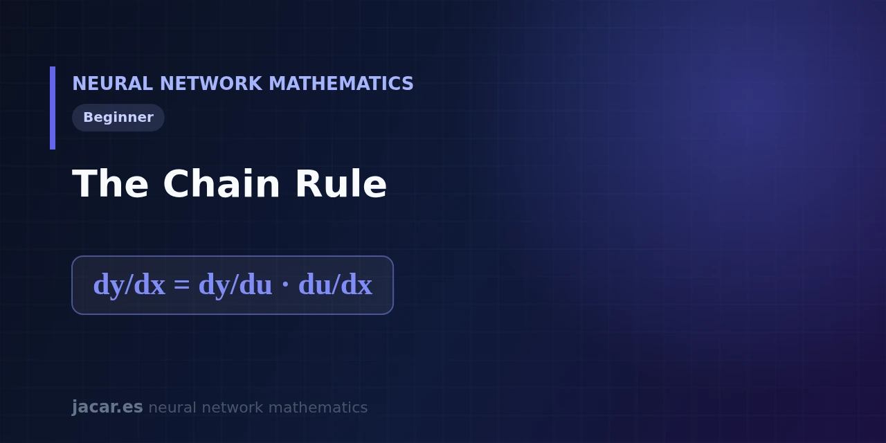
Table of contents
The chain rule is the calculus tool that lets you differentiate composite functions, and without it backpropagation would not exist. When one quantity depends on another that in turn depends on a third, the chain rule links those dependencies by multiplying derivatives. A neural network is exactly that: a composite function with dozens or hundreds of links. That is why this result, taught in a first calculus course, is the engine that adjusts millions of weights.
The same explanation is available in Spanish.
Key takeaways
- The chain rule differentiates a composite function by multiplying the derivatives of each link: $\frac{dy}{dx} = \frac{dy}{du}\cdot\frac{du}{dx}$.
- A neural network is a composition of functions, so its gradient can only be computed by applying the chain rule.
- Backpropagation is the chain rule applied backwards, from the loss to every weight, in a single pass.
- Reusing intermediate results avoids repeating work: in a 5-layer network that saves an effort that would otherwise grow exponentially.
- With this rule, training a 175-billion-parameter network like GPT-3 is still a mechanical computation, not an impossible feat.
What is the chain rule
The chain rule answers a simple question: if $y$ changes when $u$ changes, and $u$ changes when $x$ changes, how much does $y$ change when $x$ changes? The answer is to multiply the two rates of change. In Leibniz notation it reads $\frac{dy}{dx} = \frac{dy}{du}\cdot\frac{du}{dx}$, and that compact formula holds the whole idea.
It helps to be comfortable with derivatives as a rate of change before going on, because each factor of the rule is exactly a derivative. The intuition is two meshed gears. If the first turns 3 times faster than the second, and the second turns 2 times faster than the third, the first turns 6 times faster than the third. Rates of change multiply, they do not add.
Function composition
Composing functions means applying one after another. If f and g are functions, the composition y = f(g(x)) first computes u = g(x) and then y = f(u). The output passes through two chained stages, and each stage has its own sensitivity to change.
A numerical example clarifies it. Let $g(x) = 2x$ and $f(u) = u^2$, so $y = (2x)^2 = 4x^2$. We can differentiate directly: $\frac{dy}{dx} = 8x$. Or we can use the chain rule: $\frac{dy}{du} = 2u = 4x$ and $\frac{du}{dx} = 2$, so $\frac{dy}{dx} = 4x \cdot 2 = 8x$.
Both paths agree, but the second scales to functions where differentiating in one shot is impossible.
Why it is the key to backpropagation
A neural network chains many functions together. Each layer computes $z = Wx + b$, then an activation $a = f(z)$, and that output feeds the next layer. At the end the prediction is compared with the correct answer through a loss $L$. The whole network, from input to loss, is a single composite function with as many links as operations.
To train we need the gradient $\nabla$: how the loss $L$ changes for a small change in each weight $W^{(l)}$ of each layer. That gradient crosses every intermediate layer, and the only way to compute it is to multiply the derivatives layer by layer, that is, to apply the chain rule backwards. That is backpropagation.
The algorithm became popular in 1986 with the paper by Rumelhart, Hinton and Williams in Nature, «Learning representations by back-propagating errors»[1], which showed how to obtain the gradient of every weight in a single backward pass. As Michael Nielsen puts it in his open book, «backpropagation is not just a fast algorithm for learning: it gives us detailed insight into how changing the weights changes the network’s behaviour».
Step-by-step example
Take a minimal neuron with one weight $w$, input $x = 2$ and a quadratic activation. Define $z = w \cdot x$, $a = z^2$ and a loss $L = a$. We want $\frac{dL}{dw}$, the signal gradient descent uses to adjust $w$. We apply the chain rule across three links:
- $\frac{dL}{da} = 1$, because the loss is the activation itself.
- $\frac{da}{dz} = 2z$, the derivative of the quadratic function.
- $\frac{dz}{dw} = x = 2$, since $z = w \cdot x$.
See the derivation
Chain the three local factors together: $\frac{dL}{dw} = \frac{dL}{da}\cdot\frac{da}{dz}\cdot\frac{dz}{dw} = 1 \cdot 2z \cdot 2 = 4z$. With $w = 3$ we have $z = w\cdot x = 6$, so $\frac{dL}{dw} = 4 \cdot 6 = 24$. The gradient-descent step is $w \leftarrow w-\eta\,\frac{dL}{dw} = 3-0.1 \cdot 24 = 0.6$.
Multiplying: $\frac{dL}{dw} = 1 \cdot 2z \cdot 2 = 4z$. If the current weight is $w = 3$, then $z = 6$ and $\frac{dL}{dw} = 24$. With a learning rate $\eta = 0.1$, the new weight is $w = 3-0.1 \cdot 24 = 0.6$. The chain rule has turned three simple local derivatives into the exact instruction to reduce the error.
Each factor in the chain is a local derivative: it only looks at its own link. Backpropagation computes these local derivatives once and reuses them, which is why its cost grows linearly with the number of layers rather than exponentially.
The multivariable chain rule
In a real network every value influences many others, not just one. When $L$ depends on several intermediate variables, the chain rule generalises by summing the contributions of all paths: if $u$ affects $L$ through $p$ and $q$, then $\frac{\partial L}{\partial u} = \frac{\partial L}{\partial p}\cdot\frac{\partial p}{\partial u} + \frac{\partial L}{\partial q}\cdot\frac{\partial q}{\partial u}$. This version, with sums of products, is the one that appears in the gradient of a layer with many neurons.
The reference text Deep Learning[2] formalises this idea with Jacobian matrices: the gradient of the whole network is a product of Jacobians, one per layer. Backpropagation arranges that product from right to left so as not to repeat work, which cuts the cost from exponential to linear in the number of layers.
Frequently asked questions
Why are the derivatives multiplied and not added?
Because they measure chained rates of change, not accumulated amounts. If $y$ changes twice as fast as $u$ and $u$ changes three times as fast as $x$, then $y$ changes six times as fast as $x$. That combined factor is a product, $2 \cdot 3 = 6$, exactly as the chain rule states.
Is backpropagation the same as the chain rule?
They are inseparable but not identical. The chain rule is the mathematical result that says how to differentiate a composition. Backpropagation is the algorithm that applies that rule in an orderly, efficient way, reusing intermediate results to compute all the gradients in a single backward pass.
Conclusion
The chain rule looks like a technicality from a first calculus course, but it is the exact mechanism that makes training neural networks possible. It differentiates composite functions by multiplying links, and a network is nothing but a long composite function. Master this rule and backpropagation stops being magic and becomes arithmetic. The natural next step is to see how it fits into the mathematics behind neural networks roadmap alongside gradient descent.
Sources: [1] Deep Learning (Goodfellow, Bengio and Courville)[2], [2] Neural Networks and Deep Learning (Michael Nielsen)[3], [3] Chain rule (Wikipedia)[4], [4] Learning representations by back-propagating errors (Nature, 1986)[1].