
Mean Absolute Error (MAE) and Huber Loss
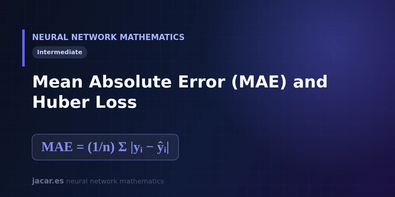
Mean absolute error measures how wrong a model is by averaging the absolute value of each error, which is why it copes so well with outliers. When an odd data point sneaks into the training set, mean squared error squares it and lets it dominate the loss; MAE, by contrast, treats it in proportion. Huber loss takes the best of both: it behaves like squared error near a correct prediction and like MAE once the error grows.
This guide explains the three ideas and when each one fits. The same explanation is available in Spanish.
Key takeaways
- The mean absolute error (MAE, or L1 loss) is the average of $\lvert y_i-\hat{y}_i\rvert$: the mean distance between prediction and reality, in the same units as the target.
- Unlike mean squared error (MSE), MAE does not square the errors, so an outlier has a linear influence and does not hijack training.
- Its weak spot is the derivative: the MAE gradient is $+1$ or $-1$ almost everywhere and does not exist at zero, which complicates fine tuning.
- Huber loss, proposed by Peter Huber in 1964, is quadratic for small errors and linear for large ones.
- The delta parameter sets the boundary between the two zones: below delta the loss is smooth; above it, robust.
What is the MAE?
Mean absolute error answers a simple question: on average, by how much is the model wrong? For each example you compute the difference between the true value $y_i$ and the prediction $\hat{y}_i$, take its absolute value so the signs do not cancel, and average all the differences over the $n$ examples. In compact notation:
$$\mathrm{MAE} = \frac{1}{n}\sum_{i=1}^{n}\lvert y_i-\hat{y}_i\rvert$$
Its great strength is interpretability. If a house-price model has an MAE of 12,000 euros, the reading is direct: on average it is 12,000 euros off the real price. That transparency makes it the first metric worth checking in a regression problem, as the scikit-learn[1] documentation notes. In deep learning MAE is also called L1 loss and is implemented directly, for example in PyTorch[2] as nn.L1Loss.
MAE versus MSE
The key difference is how they punish large errors. Mean squared error squares each difference, so an error of 100 contributes 10,000 to the sum, whereas in MAE it contributes only 100. That quadratic factor makes MSE chase outliers obsessively, which helps when every big miss is genuinely serious but hurts when the outliers are just measurement noise.
MAE, being linear, spreads its attention more evenly. Statistically, the model that minimises MAE tends towards the median of the data, which withstands up to 50% contamination before breaking down. The one that minimises MSE tends towards the mean, far more sensitive. That is why, on a set with noisy labels, MAE tends to yield more stable predictions.
The trade-off is training. Because the derivative of the absolute value is constant ($+1$ or $-1$) and jumps abruptly at zero, gradient descent takes steps of the same size whether it is near or far from the minimum. That makes it harder to refine the solution. You can review why the derivative matters in the essential differentiation rules.
Mnemonic: minimising MAE pulls the model towards the median of the data, whereas minimising MSE pulls it towards the mean. The median ignores the size of outliers, and that is exactly why it is more robust.
Huber loss, the best of both
Huber loss resolves that tension by fusing the two functions into one. For small errors it behaves like MSE, with a smooth curve that eases convergence; for large errors it switches to a linear segment like MAE, which refuses to be dragged around by outliers. Its piecewise definition, with error $r=y-\hat{y}$, is quadratic when $\lvert r\rvert \le \delta$ and linear when $\lvert r\rvert > \delta$:
$$L_\delta(r) = \begin{cases} \frac{1}{2}\,r^2 & \text{if } \lvert r\rvert \le \delta \ \delta\left(\lvert r\rvert-\tfrac{1}{2}\delta\right) & \text{if } \lvert r\rvert > \delta \end{cases}$$
The two pieces meet continuously and with a continuous derivative at the boundary, and that smooth seam is what gives Huber its balanced behaviour.
Show the derivation
The constant $\tfrac{1}{2}\delta$ in the linear branch is not arbitrary: it is chosen so the two pieces fit together. At $\lvert r\rvert=\delta$ the quadratic branch equals $\tfrac{1}{2}\delta^2$ and the linear branch equals $\delta\left(\delta-\tfrac{1}{2}\delta\right)=\tfrac{1}{2}\delta^2$, so the loss is continuous. Their derivatives match too: the quadratic branch has derivative $r$, which at $r=\delta$ equals $\delta$, and the linear branch has constant derivative $\delta$. By matching both value and slope at the boundary, Huber switches from quadratic to linear with no jump.
Peter Huber introduced it in his 1964 paper on robust estimation. As he later summed up the spirit of the whole approach, «robustness signifies insensitivity to small deviations from the assumptions». That idea, applied to a loss function, is exactly what we want: an objective that does not break because a handful of examples fall outside expectations. Wikipedia[3] records the full formulation and its smooth variant, the pseudo-Huber loss.
The delta parameter
Delta is the dial that decides where the quadratic zone ends and the linear one begins. With a large delta almost every error falls inside the quadratic segment and Huber loss looks like MSE; with a small delta almost everything falls in the linear segment and it looks like MAE. The default in PyTorch for nn.HuberLoss is delta = 1.0, whereas scikit-learn’s HuberRegressor uses an equivalent parameter, epsilon, defaulting to 1.35, chosen to keep around 95% statistical efficiency when the data are normal.
Choosing delta is, in practice, deciding above what size we consider an error to be an outlier that should not dominate. A good habit is to set it relative to the scale of the typical error. If that typical error hovers around a certain value, delta should sit slightly above it, so only genuine outliers enter the robust segment. It is one more hyperparameter worth tuning by validation.
When to use each one
The practical rule is short. If the data are clean and every large error must be penalised heavily, MSE remains the natural choice and the most direct to optimise. If you suspect outliers or noisy labels and want an interpretable metric, MAE is more honest. And if you want robustness without giving up smooth training, Huber loss is the middle ground, widely used in regression and in object detection.
This article is part of the mathematics behind neural networks roadmap, where it sits right after mean squared error.
Frequently asked questions
Is MAE the same as L1 loss?
Yes. L1 loss is the name MAE takes in the deep learning context, because it rests on the L1 norm (the sum of absolute values). In libraries such as PyTorch it appears as L1Loss, and it computes exactly the average of the absolute value of the errors.
Why is MAE more robust than MSE?
Because it does not square the errors. An outlier contributes to the loss in proportion to its size, not its square, so it cannot dominate training. The resulting model orients towards the median of the data, which is far more stable against contamination than the mean.
Which delta should I use in Huber loss?
It depends on the scale of your errors. A good starting point is the 1.0 that PyTorch uses by default, or scikit-learn’s 1.35 if you work with roughly normal data. Ideally treat it as a hyperparameter and tune it by cross-validation according to how many residuals you want to count as outliers.
Conclusion
Mean absolute error and Huber loss share a single philosophy: never let a few huge errors hijack learning. MAE achieves it with a linear, interpretable and robust metric, at the cost of an awkward derivative. Huber loss recovers the smoothness of MSE in the central zone and keeps the robustness of MAE in the tails, with delta as the needle of the scale. Choosing well among the three functions is a design decision that depends on how much noise you expect in your data.