Binary Cross-Entropy
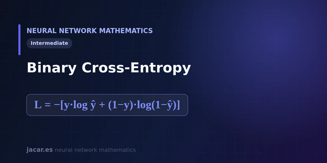
Table of contents
- Key takeaways
- What is binary cross-entropy?
- Formula and its link to the sigmoid
- Interpretation as log-likelihood
- Derivative and why it pairs with the sigmoid
- Numerical example
- Frequently asked questions
- what is the difference between binary and categorical cross-entropy?
- why not use mean squared error for classification?
- what happens if the prediction is exactly 0 or 1?
- Conclusion
- Sources
Binary cross-entropy is the function that measures how wrong a two-class classifier is. When a network ends in a sigmoid neuron, that neuron returns a probability between 0 and 1. Binary cross-entropy compares that probability with the true label, which can only be 0 or 1. The result is a number that training tries to shrink.
Understanding its formula, where it comes from and why it fits the sigmoid so well clears up much of how a network learns to say "yes" or "no". The same explanation is available in Spanish.
Key takeaways
- Binary cross-entropy is the default loss function when the output is a single-class probability:
L = −[y·log(ŷ) + (1−y)·log(1−ŷ)]. - Only one of the two terms is active per example, because the label
yis 0 or 1 and cancels the other summand. - It comes from maximum likelihood: minimising this loss is the same as maximising the probability the network assigns to the real data.
- It punishes confident mistakes hard. Predicting 0.01 when the answer was 1 costs 4.6, almost forty times more than a lukewarm 0.5 miss.
- Combined with the sigmoid, its derivative with respect to the input collapses to
ŷ − y, a clean gradient that makes training stable.
What is binary cross-entropy?
Binary cross-entropy, also called log loss, is the loss function used when a model must decide between two options: spam or not spam, tumour or healthy tissue, click or no click. The network produces a single probability ŷ (the probability that the class is 1), and we have the true label y, which is 1 if the example belongs to that class and 0 otherwise.
The idea is to measure surprise. If the label is 1 and the network predicts 0.99, there is almost no surprise and the loss is tiny. If the label is 1 and the network predicts 0.02, the surprise is huge and the loss shoots up.
That asymmetry comes from information theory: the logarithm measures the bits needed to correct a wrong prediction, as the cross-entropy article on Wikipedia[1] explains. It is the special two-class case of the general cross-entropy we study in the mathematics of neural networks roadmap.
Formula and its link to the sigmoid
The formula for a single example is:
$$\mathcal{L} = -[y\log(\hat{y}) + (1-y)\log(1-\hat{y})]$$
The trick is that $y$ is only 0 or 1, so one term vanishes in every example. If $y=1$, the loss becomes $-\log(\hat{y})$. If $y=0$, it becomes $-\log(1-\hat{y})$. It is a compact way to write two cases in a single line.
The value $\hat{y}$ almost always comes from a sigmoid neuron, $\hat{y} = \sigma(z) = \frac{1}{1+e^{-z}}$, where $z = \mathbf{W}x+b$ is the weighted sum of the last layer. The sigmoid guarantees that $\hat{y}$ lies between 0 and 1, exactly the range the logarithm needs so it does not break. That is why this pair, sigmoid plus binary cross-entropy, is the standard output of any two-class classifier, as the PyTorch reference for BCELoss[2] documents.
Interpretation as log-likelihood
Where does this specific formula come from? It is not arbitrary: it appears on its own when we apply maximum likelihood. We model each label as a biased coin (a Bernoulli distribution) whose probability of landing on 1 is $\hat{y}$. The probability of observing the true label $y$ is then $\hat{y}^{y}(1-\hat{y})^{1-y}$.
Training means choosing the weights that maximise that probability over all the data. Because multiplying small probabilities one after another leads to tiny, unstable numbers, we take the logarithm, which turns the product into a sum, and flip the sign to get something to minimise. Applying $\log$ to $\hat{y}^{y}(1-\hat{y})^{1-y}$ gives exactly $y\log(\hat{y}) + (1-y)\log(1-\hat{y})$.
Minimising binary cross-entropy is therefore the same as maximising likelihood. As the reference book by Goodfellow, Bengio and Courville puts it, «most modern neural networks are trained using maximum likelihood».
Derivative and why it pairs with the sigmoid
Here is the elegant part. To train, we need the gradient of the loss with respect to $z$, the sigmoid’s input. If we differentiate the loss only with respect to $\hat{y}$, the result is awkward: $\frac{\partial \mathcal{L}}{\partial \hat{y}} = -\frac{y}{\hat{y}} + \frac{1-y}{1-\hat{y}}$, with a denominator that blows up as $\hat{y}$ approaches 0 or 1.
The magic happens when we apply the chain rule with the derivative of the sigmoid, which is $\sigma'(z) = \hat{y}(1-\hat{y})$. That factor cancels exactly the troublesome denominators, and everything reduces to:
$$\frac{\partial \mathcal{L}}{\partial z} = \hat{y}-y$$
The gradient $\hat{y}-y$ only comes out this clean when the sigmoid and binary cross-entropy are differentiated together. If you evaluate the sigmoid and the logarithm separately you can hit $\log(0)$ and lose precision, so in practice you should use the fused version the libraries provide.
Show the derivation
Start from $\mathcal{L} = -[y\log(\hat{y}) + (1-y)\log(1-\hat{y})]$ with $\hat{y} = \sigma(z)$. Differentiating with respect to $\hat{y}$ gives $\frac{\partial \mathcal{L}}{\partial \hat{y}} = -\frac{y}{\hat{y}} + \frac{1-y}{1-\hat{y}} = \frac{\hat{y}-y}{\hat{y}(1-\hat{y})}$. The chain rule adds the factor $\frac{\partial \hat{y}}{\partial z} = \sigma'(z) = \hat{y}(1-\hat{y})$. Multiplying, the $\hat{y}(1-\hat{y})$ in the numerator and denominator cancels, leaving $\frac{\partial \mathcal{L}}{\partial z} = \hat{y}-y$.
The gradient is the difference between what the network predicted and what it should have predicted. There are no dangerous divisions and no terms that explode. That is why serious libraries fuse the two operations into a single stable function, such as BCEWithLogitsLoss, instead of chaining sigmoid and logarithm separately. This clean result is the practical reason binary cross-entropy has almost entirely replaced mean squared error in classifiers.
Numerical example
Let us look at three predictions to feel the scale of the penalties. Suppose the correct label is $y=1$ in all three cases.
- The network predicts $\hat{y} = 0.9$ (confident hit): $\mathcal{L} = -\log(0.9) \approx 0.105$.
- The network predicts $\hat{y} = 0.5$ (total doubt): $\mathcal{L} = -\log(0.5) \approx 0.693$.
- The network predicts $\hat{y} = 0.1$ (confident miss): $\mathcal{L} = -\log(0.1) \approx 2.303$.
The contrast is huge: being confidently wrong costs about twenty-two times more than being confidently right (2.303 versus 0.105). That penalty shape is what pushes the network to calibrate its probabilities well, not just to get the class right.
When the label is $y=0$ the calculation flips. If the network predicts $\hat{y} = 0.2$, the active term is $-\log(1-0.2) = -\log(0.8) \approx 0.223$. For a full batch, the final loss is the mean of all these quantities. If our batch held those four values (0.105, 0.693, 2.303 and 0.223), the mean loss would be roughly 0.831.
That is the number gradient descent tries to reduce at each step with learning rate $\eta$.
Frequently asked questions
what is the difference between binary and categorical cross-entropy?
The binary version is used when there are two classes and a single output probability from a sigmoid. The categorical version is used when there are three or more classes, with a softmax producing one probability per class. The binary case is the special two-option case of the categorical one, and both share the same negative-logarithm idea.
why not use mean squared error for classification?
Because with the sigmoid, squared error produces an almost flat loss surface in the regions where the network is badly wrong, which stalls learning. Binary cross-entropy keeps a strong gradient exactly there, $\hat{y}-y$, so it corrects big mistakes.
what happens if the prediction is exactly 0 or 1?
The logarithm of 0 is minus infinity, so the loss would break. Libraries avoid it by clipping ŷ to a range such as [1e−7, 1 − 1e−7] or, better, computing the loss directly from z with a numerically stable version that never evaluates log(0).
Conclusion
Binary cross-entropy is not a whimsical formula but the direct translation of a simple question: what probability did the network give to the correct answer? It comes from maximum likelihood, fits the sigmoid naturally and hands you a gradient as simple as $\hat{y}-y$. With those three pieces you have the engine of almost any two-class classifier. The natural next step is to see how it generalises to more than two classes in the softmax function.
Sources: [1] Deep Learning (Goodfellow, Bengio and Courville)[3], [2] Cross-entropy (Wikipedia)[1], [3] PyTorch, BCELoss[2], [4] Neural Networks and Deep Learning (Michael Nielsen)[4].