Gradient Descent
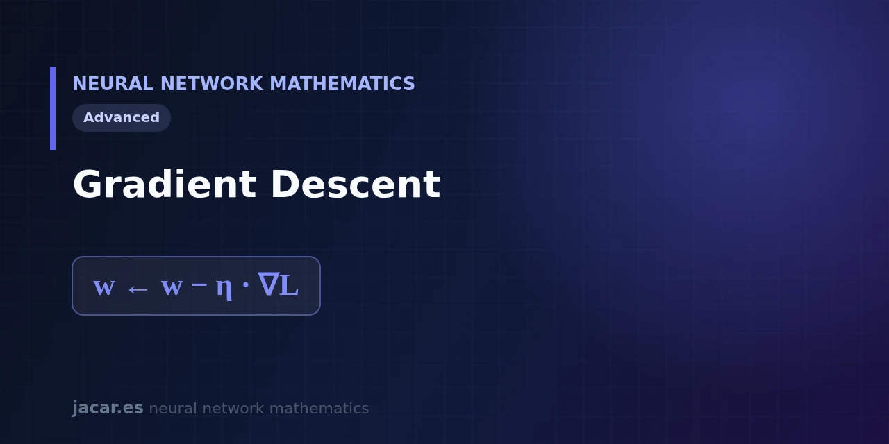
Table of contents
- Key takeaways
- What is gradient descent?
- The weight update rule
- The role of the gradient
- The mountain analogy
- Step-by-step example
- Frequently asked questions
- Why do we subtract the gradient instead of adding it?
- What happens if the learning rate is too high?
- Does gradient descent always find the best solution?
- Conclusion
- Sources
Gradient descent is the engine that makes a neural network learn. Every time a model improves a prediction, it applies the same idea under the surface. Measure how wrong it is, work out which way that error grows, and move the weights in the opposite direction.
This article explains that mechanism with the update rule, the role of the gradient, and a step-by-step numeric example. The same explanation is available in Spanish.
Key takeaways
- Gradient descent is an optimization algorithm that adjusts a network’s weights to reduce the loss function $L$.
- The core rule is $w \leftarrow w-\eta \nabla L$: each weight moves a little in the direction opposite to the gradient.
- The gradient $\nabla L$ points toward where the error grows fastest, which is why we subtract it, to go down rather than up.
- The learning rate $\eta$ sets the step size: too large and training blows up, too small and it takes forever.
- Augustin-Louis Cauchy formulated the method in 1847, and today it trains 175-billion-parameter models like GPT-3.
What is gradient descent?
Gradient descent is an iterative method for finding the minimum of a function. In a neural network that function is the loss $L$, which measures the distance between what the model predicts and the correct answer. Training means searching for the weights $W$ and biases $b$ that make $L$ as small as possible.
The idea: you start with random weights, measure how wrong you are, and correct a little. You repeat that cycle thousands or millions of times.
As Sebastian Ruder puts it, «gradient descent is the preferred way to optimize neural networks and many other machine learning algorithms but is often used as a black box». This article opens that box. To place it in the bigger picture, you can return to the roadmap of the mathematics behind neural networks.
The weight update rule
The whole mechanism fits on one line:
$$w \leftarrow w-\eta \nabla L$$
Read it like this: the new value of weight $w$ is its current value minus the learning rate $\eta$ times the gradient of the loss with respect to that weight. The arrow means we assign the result back into $w$. In a network with millions of parameters, this operation applies to every one of them at every step.
The minus sign is the important part. The gradient points uphill, so subtracting it takes us downhill, toward less error. Computing those gradients layer by layer is exactly what backpropagation does.
The minus sign is not a detail: if you added the gradient instead of subtracting it you would have gradient ascent, and the model would get worse at every step.
The role of the gradient
The gradient $\nabla L$ is a vector with one partial derivative per weight. Each component answers the question: if I nudge this weight a touch, how much does the error rise or fall? Together, all those answers form the direction of steepest ascent of the loss.
Because we want to go down, we take the opposite direction. That is where the name comes from: we descend along the gradient. When the gradient gets close to zero, the slope is nearly flat and we have reached a minimum, the point where the error stops improving.
The mountain analogy
Imagine you are on a mountainside in thick fog and want to reach the valley. You cannot see the bottom, but you can feel the slope under your feet. A reasonable strategy is to take a step in the steepest downhill direction, look again, and repeat.
That is exactly gradient descent. The mountain is the loss surface, your position is the current weights, and the slope is the gradient. The size of each step is the learning rate $\eta$.
Take huge strides and you may overshoot the valley and land higher on the far side; take tiny steps and you will get there, but after far more iterations. In practice people try values like $0.1$, $0.01$, or $0.001$ until they find one that descends without destabilizing.
There is one honest caveat: a network’s surface is not a clean bowl-shaped valley. It is non-convex: valleys and saddles are spread all over the surface. Gradient descent finds a good minimum, but does not guarantee the best of all. In large networks that is enough to produce excellent models.
Step-by-step example
Let us see it with a tiny single-weight loss: $L(w) = w^2$. Its derivative is $\nabla L = 2w$, so the rule becomes $w \leftarrow w-\eta \cdot 2w$. We set $\eta = 0.1$ and start at $w = 4$.
- Starting point: $w = 4$, loss $L = 16$.
- First update: $w \leftarrow 4-0.1 \cdot 2 \cdot 4 = 4-0.8 = 3.2$.
- Second: $w \leftarrow 3.2-0.1 \cdot 2 \cdot 3.2 = 3.2-0.64 = 2.56$.
- Third: $w \leftarrow 2.56-0.512 = 2.048$.
The weight approaches 0 (the true minimum) more and more slowly, because the gradient shrinks as we get closer. After about 30 iterations we would be practically at the bottom. This same dance happens at once for every weight in a network, coordinated by the chain rule. For groups of examples, small-batch variants are used: between 50 and 256 samples per step.
See the following iterations
Each step multiplies the weight by $0.8$, because $w-0.1 \cdot 2w = 0.8\,w$. So the sequence is geometric: $w_n = 4 \cdot 0.8^{\,n}$. Continuing from $2.048$ we get $1.6384$, then $1.31072$, then $1.048576$… After 30 steps, $w \approx 4 \cdot 0.8^{30} \approx 0.005$, practically at the minimum.
Frequently asked questions
Why do we subtract the gradient instead of adding it?
Because the gradient points toward where the loss grows fastest. Our goal is to reduce the error, not increase it, so we move in the opposite direction. Adding it would be gradient ascent: it would make the model worse step by step.
What happens if the learning rate is too high?
Training becomes unstable. With steps that are too large, the model bounces from one side of the valley to the other without settling, and the loss can grow out of control until it diverges. That is why it is tuned carefully and sometimes reduced over the course of training.
Does gradient descent always find the best solution?
Not always. A network’s error surface is non-convex, with multiple local minima and saddle points. The method is guaranteed to reach a minimum, but not necessarily the global one. In practice, the minima it finds are usually good enough.
Conclusion
Gradient descent reduces learning to a clear recipe: measure the error, compute the gradient, and take a small step downhill with w ← w − η · ∇L. All the later sophistication, from momentum to Adam, is just smarter ways of choosing that direction and step size. The natural next step is to understand how the gradient is computed in each layer with partial derivatives and the gradient.