Dropout and Its Mathematical Interpretation
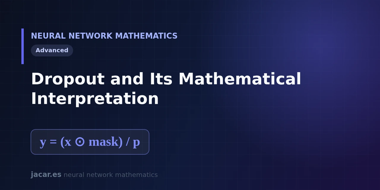
Table of contents
Dropout is the most famous form of regularization in deep learning: during training it switches neurons off at random so the network cannot depend on any single one. The idea looks like a blunt trick, but it has a precise mathematical reading.
Turning units off amounts to training and averaging a gigantic number of smaller networks, and the 1/p scaling keeps the arithmetic consistent between training and inference. This guide takes that mechanism apart step by step. The same explanation is available in Spanish.
Key takeaways
- Dropout switches each neuron in a layer off with probability
1 - pon every training step;pis the retention probability, and a typical value in hidden layers is 0.5. - By turning units off, the network cannot rely on any single neuron and learns more redundant representations, which reduces overfitting.
- Inverted dropout divides the surviving activations by
pduring training, so nothing needs adjusting at inference time. - Mathematically, dropout trains an implicit ensemble of up to $2^n$ subnetworks that share weights, and at inference it approximates their average.
- The technique was introduced by Srivastava, Hinton and their co-authors in 2014, following earlier 2012 work on the co-adaptation of feature detectors.
What is dropout?
Dropout is a regularization technique designed to fight overfitting, the same problem that L1 and L2 regularization tackle by another route. In a dense network, each layer computes z = Wx + b and applies an activation a = f(z). Dropout adds a step: before passing a to the next layer, it zeroes a randomly chosen fraction of its components on every training step.
The intuition is this. If a neuron knows that its companions may vanish at any moment, it cannot specialize in fixing a specific neighbour’s mistakes. The network is forced to spread information out and to build detectors that work on their own. As Srivastava and his co-authors put it, «the key idea is to randomly drop units (along with their connections) from the neural network during training».
The central parameter is the retention probability p: the chance that a neuron survives a step. With p = 0.5, half the neurons are switched off on average at each iteration. The convention for input layers is a higher value, close to 0.8, so as not to throw away too much of the raw signal.
How it drops units at random
Formally, on each step dropout generates a mask vector $m$ with the same dimension as the activation $a$. Each component of the mask is a Bernoulli variable: it is 1 with probability $p$ and 0 with probability $1-p$. The layer output is computed by multiplying the activation elementwise by that mask:
$$m \sim \operatorname{Bernoulli}(p), \qquad y = a \odot m$$
The symbol $\odot$ is the Hadamard product, componentwise multiplication. Where the mask is 0, the neuron is silenced for that step; where it is 1, it passes through untouched. On the next batch a fresh mask is drawn, so the active subnetwork changes constantly.
This sampling has a direct effect on the statistics of the signal. If an activation had expected value $a$, after the mask its expected value becomes $p \cdot a$, because it survives only a fraction $p$ of the time. That drop in scale is exactly the problem the inverted scaling solves.
Inverted dropout scaling
The network trains with activations reduced on average to $p \cdot a$, but at inference we want to use every neuron. If we corrected nothing, the average input to the next layer would be $1/p$ times larger at inference than in training, and the network would receive signals of a scale it never saw. There are two ways to fix this.
The original version multiplied the activations by $p$ at inference. The modern version, called inverted dropout, does the opposite and more convenient thing: it divides by $p$ during training, leaving inference clean. The full formula is the one on the cover:
$$y = \frac{x \odot m}{p}$$
The $1/p$ factor is not arbitrary: it is exactly the inverse of the retention probability, so it cancels the scale reduction the mask introduces and leaves the expected value intact.
With this $1/p$ factor, the expected value of each component returns to $a$: we multiply by $p$ when applying the mask and divide by $p$ when scaling, so the mean is preserved.
See why the mean is preserved
Let $a$ be the expected value of an activation before dropout. The mask lets it through with probability $p$ and zeroes it with probability $1-p$, so $\mathbb{E}[a \odot m] = p \cdot a$. Inverted dropout divides by $p$, hence $\mathbb{E}\!\left[\tfrac{a \odot m}{p}\right] = \tfrac{1}{p} \cdot p \cdot a = a$. The mean returns to its original value, which is why inference needs no adjustment.
In code, a dropout layer trained with $p = 0.5$ multiplies the surviving activations by 2:
import torch

def inverted_dropout(a, p=0.5, training=True):
    if not training:
        return a
    mask = (torch.rand_like(a) < p).float()  # 1 with prob p, 0 with prob 1-p
    return a * mask / p                       # scaling 1/p preserves the mean
That is why torch.nn.Dropout needs no change when you switch to evaluation: with model.eval() the layer becomes the identity and returns the input untouched. The scaling was already paid for during training.
Dropout as an implicit ensemble
Here is the deeper reading. A layer with n neurons has $2^n$ possible on/off patterns. Each mask selects a different subnetwork, and all of those subnetworks share the same weights W. Training with dropout amounts to training, a little on each step, that enormous family of smaller networks.
At inference we would like to average the predictions of all subnetworks, the standard ensemble recipe for raising accuracy. Computing $2^n$ passes is infeasible, but dropout offers a cheap approximation: use the full network once with the scaled weights. That single pass approximates the geometric mean of the ensemble’s predictions, which is why dropout is described as an implicit ensemble. The connection to classic bagging is direct, with the difference that here the models are not independent but share parameters.
This reading explains why dropout works well with large networks: the more neurons, the larger the implicit ensemble and the more robust the resulting average. It also explains why it pays to combine it with other stability techniques, such as batch normalization, although their interaction demands care with the order of the layers.
Training versus inference
It helps to pin down the asymmetry between the two phases, because that is where most mistakes happen:
- Training: a Bernoulli mask is drawn per batch, neurons are switched off at random, and the result is divided by
pto preserve the scale. Each batch trains a different subnetwork. - Inference: nothing is switched off. The full network processes the input once and, since the scaling was already applied, there is no extra factor to add.
Forgetting to put the model in evaluation mode is a common bug: if dropout stays active during validation, the predictions become noisy and the metrics fluctuate for no apparent reason. The regularizing effect also has a cost: because each step sees a mutilated network, training with dropout needs more epochs to converge, sometimes 1.5 to 2 times more. In exchange, the gap between the training error and the validation error narrows, which is exactly what we want.
Frequently asked questions
What value of p should I use?
It depends on the layer. In the hidden layers of a dense network, p = 0.5 is the classic starting point and almost always reasonable. In input layers a higher retention value is used, between 0.8 and 0.9, so as not to discard too much raw information. If the network is small or already generalizes well, it is better to raise p or drop the technique, because too much of it can cause underfitting.
Why divide by p instead of multiplying?
They are two equivalent conventions aiming at the same thing: making the expected value of the activations equal in training and inference. The original version multiplied by p at inference. Inverted dropout divides by p in training, which leaves inference without any adjustment. The second option won out because it simplifies deployment code, and it is the default in PyTorch and Keras.
Does dropout help in any network?
Not automatically. It works well in large dense layers, where there is plenty of redundancy to exploit. In convolutional layers its effect is smaller, because neighbouring pixels are correlated, and variants such as spatial dropout are the default choice there. In modern architectures with batch normalization, dropout sometimes adds little or even gets in the way, so its use is decided by measurement, not by habit.
Conclusion
Dropout looks like a hammer blow: it switches neurons off at random. Behind it sits an elegant idea, training an ensemble of $2^n$ weight-sharing subnetworks at once and approximating their average with a single pass. The 1/p scaling is what keeps training and inference consistent, and understanding that factor avoids the most common bugs. To place this technique within the full route, see the mathematics behind neural networks roadmap.