Backpropagation: The Intuition
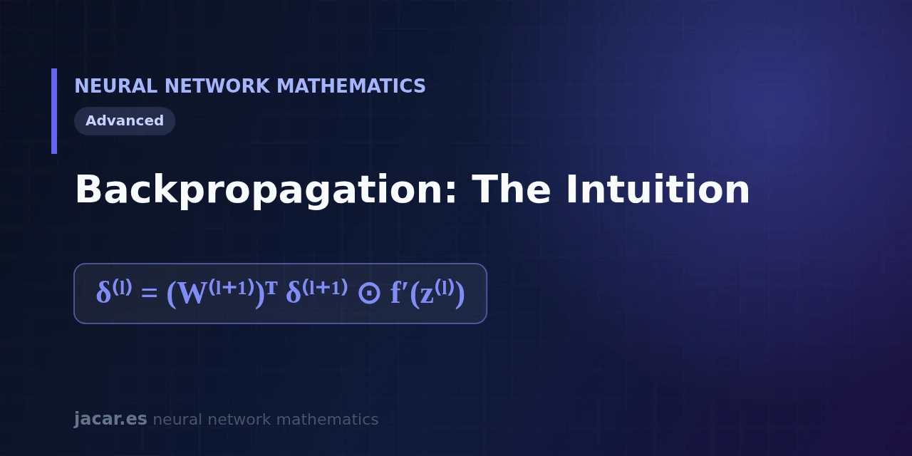
Table of contents
- Key takeaways
- What is backpropagation?
- Assigning blame for the error
- The gradient flowing backwards
- Why it is so efficient
- A preview of the derivation
- Frequently asked questions
- Is backpropagation the same as gradient descent?
- Why is it called backward propagation?
- Do I need to know calculus to understand it?
- Conclusion
- Sources
Backpropagation is the algorithm that shares out the blame for the error among all the weights of a neural network so it knows how to adjust them. Instead of trying random changes, it propagates an error signal from the output back to the input, layer by layer. A single pass computes how much each weight contributed to the final mistake.
That intuition, sharing responsibility backwards, is what made training deep networks practical. The same explanation is available in Spanish.
Key takeaways
- Backpropagation computes the gradient of every weight by propagating the error from the output to the input in a single backward pass.
- The core idea is assigning blame: each neuron receives an error signal
δthat measures how much responsibility it holds in the final mistake. - That signal propagates through the formula
δ⁽ˡ⁾ = (W⁽ˡ⁺¹⁾)ᵀ δ⁽ˡ⁺¹⁾ ⊙ f'(z⁽ˡ⁾), combining the next layer’s weights and the activation’s derivative. - Efficiency is the key: reusing intermediate computations cuts the cost from exponential to linear in the number of layers.
- Thanks to that efficiency, training a 175-billion-parameter network like GPT-3 remains a mechanical computation rather than an impossible task.
What is backpropagation?
Backpropagation is the method that lets a neural network learn from its mistakes. After the network makes a prediction through forward propagation, we compare its output with the correct answer and measure the mistake with a loss function L. The question then is: how much should each weight W change to reduce that mistake? Backpropagation answers that question for every weight at once.
The name says it all: propagation backwards. Information flows forward to produce the prediction, and the error signal flows backward to share out responsibility. The algorithm became popular in 1986 with the paper by David Rumelhart, Geoffrey Hinton and Ronald Williams in Nature, «Learning representations by back-propagating errors»[1], which showed how to obtain the gradient ∇ of every weight in a single pass. As Michael Nielsen puts it in his open book, «what’s clever about backpropagation is that it enables us to simultaneously compute all the partial derivatives using just one forward pass through the network, followed by one backward pass».
Assigning blame for the error
The best way to understand backpropagation is to think of it as sharing out blame. When the network gets it wrong, the final error is the responsibility of thousands of weights that collaborated in the prediction. Some pushed in the right direction and others in the wrong one, and each deserves a different share of the blame.
To formalise that idea we define a quantity δ (delta) for each neuron: it is the error signal, the sensitivity of the loss to a change in that neuron’s weighted input z = Wx + b. A neuron with a large δ weighed heavily on the mistake and needs a big adjustment; one with δ near zero barely contributed and is left almost untouched. Picture a team of 10 people where a project goes wrong: not everyone failed equally, and δ is precisely the share of responsibility that falls on each. That sharing is possible thanks to the chain rule, which links the local derivatives from layer to layer.
The gradient flowing backwards
The sharing starts at the output layer, where the error is direct: we compare the prediction with the correct answer. From there, the $\delta$ signal steps back one layer at a time. The formula that governs that step is the one on the cover:
$$\delta^{(l)} = \left(\mathbf{W}^{(l+1)}\right)^{\top} \delta^{(l+1)} \odot f'(\mathbf{z}^{(l)})$$
Every symbol has an intuitive reading. The term $\left(\mathbf{W}^{(l+1)}\right)^{\top}\delta^{(l+1)}$ takes the blame from the next layer and shares it backwards through the same weights that propagated it forward, but transposed: the information now travels in the opposite direction.
The symbol $\odot$ is the elementwise product, and $f'(\mathbf{z}^{(l)})$ is the derivative of the activation function. That last factor acts like a gate: if the neuron was in a flat region of its activation, its derivative is nearly zero and blocks the signal. That is why saturated activations slow learning down.
That factor $f'(\mathbf{z}^{(l)})$ is the origin of the vanishing-gradient problem. In the flat regions of a saturated activation its value falls close to $0$ and switches off the error signal before it reaches the earliest layers.
Once we have $\delta$ in each layer, the gradient of a weight is the product of the error signal of the receiving neuron and the activation of the sending neuron. With that gradient, gradient descent updates the weight: $\mathbf{W}=\mathbf{W}-\eta\cdot\nabla$, where $\eta$ is the learning rate. If in one layer $\delta = 0.5$ and the incoming activation is $a = 2$, the gradient of that weight is $1.0$, and with $\eta = 0.1$ the weight drops by $0.1$. The same computation happens in parallel for every weight in the network.
Why it is so efficient
Backpropagation is not the only way to compute the gradient, but it is the fastest by a huge margin. The naive alternative would be to perturb each weight separately, run the whole network forward again and measure how the loss changes. In a network with a million weights that would demand a million full passes per update, which is unworkable.
The key is reusing the work. By propagating δ from right to left, each layer builds on the already-computed result of the layer behind it, instead of starting from scratch. That reuse is what cuts the cost from exponential to linear in the number of layers: a single backward pass yields every gradient.
The reference book by Goodfellow, Bengio and Courville[2] describes it as an orderly application of dynamic programming over the computation graph. It is the difference between training a 50-layer network in seconds or never being able to train it at all.
A preview of the derivation
Everything above is the intuition; the formal derivation is left for the next article. There we will obtain the formula δ⁽ˡ⁾ = (W⁽ˡ⁺¹⁾)ᵀ δ⁽ˡ⁺¹⁾ ⊙ f'(z⁽ˡ⁾) by applying the chain rule term by term, starting from partial derivatives and the gradient and arriving at the four fundamental equations of backpropagation.
For now it is enough to keep three ideas in mind. The error signal δ measures each neuron’s blame. That blame propagates backwards by multiplying by the transposed weights and by the activation’s derivative. Everything is computed in a single pass.
With those three pillars, the equations will stop looking like a puzzle. It also fits into the wider mathematics behind neural networks roadmap.
Frequently asked questions
Is backpropagation the same as gradient descent?
No, they are two complementary pieces. Backpropagation computes the gradient, that is, the direction and magnitude of the change that reduces the error for each weight. Gradient descent is what uses that gradient to update the weights by taking a small step. One computes the signal and the other applies it; together they form the training loop.
Why is it called backward propagation?
Because the error signal travels in the opposite direction to the prediction. During forward propagation the data enters through the first layer and leaves through the last. During backpropagation, the blame for the error starts at the last layer and steps back towards the first, reusing the same weights but transposed to share out responsibility.
Do I need to know calculus to understand it?
The idea of a derivative as a rate of change and the chain rule are enough. You do not need to solve complicated integrals: backpropagation only multiplies and adds simple local derivatives, layer by layer.
Conclusion
Backpropagation stops being magic once you see it for what it is: an orderly sharing of the blame for the error among all the weights. The δ signal travels backwards, is multiplied by the transposed weights and by the activation’s derivative, and in a single pass delivers the full gradient. That efficiency is what underpins all of modern deep learning. The natural next step is to see where this piece fits in the mathematics behind neural networks roadmap and then tackle the formal derivation.
Sources: [1] Learning representations by back-propagating errors (Nature, 1986)[1], [2] Deep Learning (Goodfellow, Bengio and Courville)[2], [3] Neural Networks and Deep Learning (Michael Nielsen)[3], [4] Backpropagation (Wikipedia)[4].