Backpropagation: The Step-by-Step Derivation
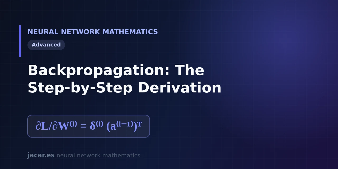
Table of contents
- Key takeaways
- Preparation: notation and the chain rule
- The error of the output layer
- Propagating the error backward
- Gradients of weights and biases
- The four equations of backpropagation
- Frequently asked questions
- Why do we multiply by the transpose of the weights?
- How is backpropagation different from gradient descent?
- Do I need to store the forward-pass activations?
- Conclusion
- Sources
Updated: 2026-10-19
Backpropagation is not magic; it is the chain rule applied in the right order. Training a network means moving each weight in the direction that reduces the error, and for that you need the gradient of the loss with respect to every parameter. Computing it weight by weight would be prohibitively expensive; backpropagation obtains all of it in a single backward pass.
This guide derives that process step by step until we reach the four equations that summarise it. The same explanation is available in Spanish.
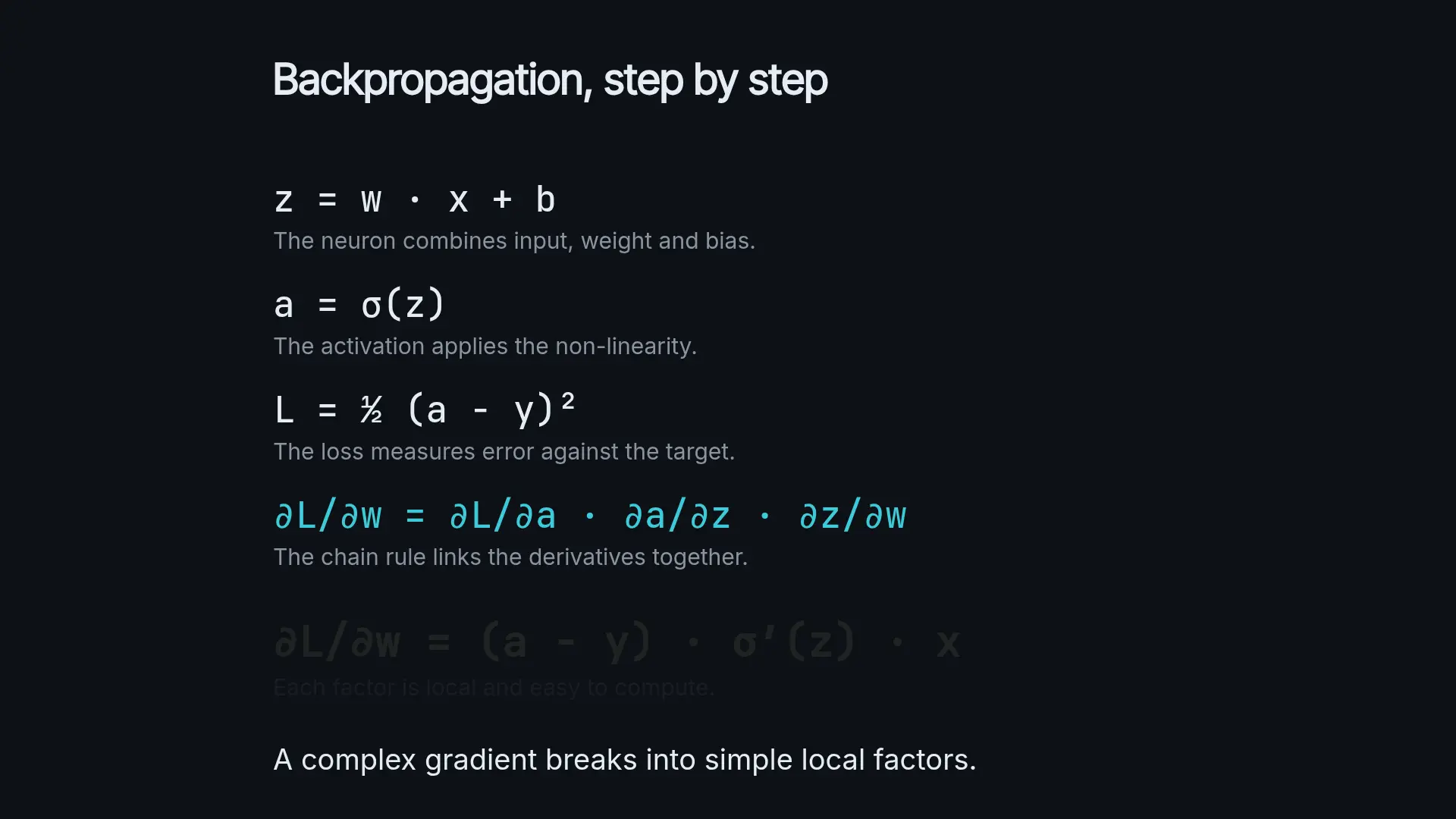
Key takeaways
- Backpropagation computes the gradient of the loss $L$ with respect to every weight and bias by applying the chain rule from the last layer back to the first.
- The starting point is the error of the output layer, $\boldsymbol{\delta}$, which combines how much the loss changes with the activation and how much the activation changes with the input $\mathbf{z}$.
- That error is propagated backward by multiplying by the transpose of the next layer’s weight matrix: $\boldsymbol{\delta}^{(l)} = \left((\mathbf{W}^{(l+1)})^{\top}\boldsymbol{\delta}^{(l+1)}\right) \odot f'(\mathbf{z}^{(l)})$.
- With $\boldsymbol{\delta}$ for each layer, the bias gradient is $\boldsymbol{\delta}$ itself and the weight gradient is $\boldsymbol{\delta}^{(l)}(\mathbf{a}^{(l-1)})^{\top}$.
- The whole algorithm fits in four equations and a single pair of passes, one forward and one backward, published by Rumelhart, Hinton and Williams in 1986.
Preparation: notation and the chain rule
Before deriving anything it helps to fix the notation, the same used in the roadmap of the mathematics of neural networks. Each layer $l$ takes the activations of the previous layer, computes a weighted sum and applies an activation function:
$$\begin{aligned} \mathbf{z}^{(l)} &= \mathbf{W}^{(l)}\mathbf{a}^{(l-1)} + \mathbf{b}^{(l)} \ \mathbf{a}^{(l)} &= f(\mathbf{z}^{(l)}) \end{aligned}$$
Here $\mathbf{W}^{(l)}$ is the weight matrix, $\mathbf{b}^{(l)}$ the bias vector, $\mathbf{z}^{(l)}$ the weighted input and $\mathbf{a}^{(l)}$ the activation. The network input is $\mathbf{a}^{(0)} = \mathbf{x}$ and the final output is $\mathbf{a}^{(L)}$ in the last layer. The loss $L$ compares that output with the correct answer.
The tool that connects everything is the chain rule. If the loss depends on $\mathbf{a}$, which depends on $\mathbf{z}$, which depends on $\mathbf{W}$, then the derivative of the loss with respect to $\mathbf{W}$ is the product of those chained derivatives. Backpropagation is that chain traversed from right to left so that no work is repeated. As Michael Nielsen writes in his chapter on the subject, «backpropagation gives us detailed insights into how changing the weights and biases changes the overall behaviour of the network».
The error of the output layer
The first link is the error of the last layer, defined as the sensitivity of the loss to the weighted input $\mathbf{z}$:
$$\boldsymbol{\delta}^{(L)} = \frac{\partial L}{\partial \mathbf{a}^{(L)}} \odot f'(\mathbf{z}^{(L)})$$
The symbol $\odot$ is the element-wise (Hadamard) product. The reading is intuitive: $\frac{\partial L}{\partial \mathbf{a}^{(L)}}$ measures how much the loss worsens if the output changes, and $f'(\mathbf{z}^{(L)})$ measures how much the output changes if $\mathbf{z}$ changes. Their product tells how much of the error each output neuron is responsible for.
Although we call $\boldsymbol{\delta}$ the “error”, it is not the loss itself but its sensitivity with respect to the weighted input $\mathbf{z}$. That distinction is what lets us chain layers: each $\boldsymbol{\delta}$ measures local blame, not total error.
A concrete example: with the quadratic loss $L = \tfrac{1}{2}(\mathbf{a}^{(L)}-\mathbf{y})^2$, the first factor is $\mathbf{a}^{(L)}-\mathbf{y}$, the gap between predicted and true. If the activation is the sigmoid, $f'(z) = f(z)\,(1-f(z))$, which peaks at $0.25$ and explains why deep layers learn slowly, the so-called vanishing gradient.
Propagating the error backward
Here is the heart of the algorithm. Knowing the error $\boldsymbol{\delta}^{(l+1)}$ of one layer, we want the previous layer’s without recomputing anything from scratch. The chain rule, applied through the weighted sum of the next layer, gives:
$$\boldsymbol{\delta}^{(l)} = \left((\mathbf{W}^{(l+1)})^{\top}\boldsymbol{\delta}^{(l+1)}\right) \odot f'(\mathbf{z}^{(l)})$$
Multiplying by the transpose $(\mathbf{W}^{(l+1)})^{\top}$ distributes the error of layer $l+1$ among the neurons of layer $l$ according to how much each contributed. Then the Hadamard product with $f'(\mathbf{z}^{(l)})$ filters it by the local slope of the activation. Repeating this formula from the last layer to the first yields the $\boldsymbol{\delta}$ of every layer: that is why the method is called backpropagation, because the error travels backward.
Show the derivation
Start from $\delta^{(l)}_j = \dfrac{\partial L}{\partial z^{(l)}_j}$ and chain through every input $z^{(l+1)}_k$ of the next layer, since $z^{(l+1)}_k = \sum_j W^{(l+1)}_{kj}\,f(z^{(l)}_j)+b^{(l+1)}_k$. The chain rule gives $\delta^{(l)}_j = \sum_k \dfrac{\partial L}{\partial z^{(l+1)}_k}\dfrac{\partial z^{(l+1)}_k}{\partial z^{(l)}_j} = \sum_k \delta^{(l+1)}_k\,W^{(l+1)}_{kj}\,f'(z^{(l)}_j)$. Rewriting the sum $\sum_k \delta^{(l+1)}_k\,W^{(l+1)}_{kj}$ as the matrix-vector product $(\mathbf{W}^{(l+1)})^{\top}\boldsymbol{\delta}^{(l+1)}$ and factoring out $f'(z^{(l)}_j)$ with the Hadamard product yields $\boldsymbol{\delta}^{(l)} = \left((\mathbf{W}^{(l+1)})^{\top}\boldsymbol{\delta}^{(l+1)}\right) \odot f'(\mathbf{z}^{(l)})$.
This recursion is what makes the algorithm efficient. Instead of computing an independent derivative for each of the, say, millions of weights, we reuse the $\boldsymbol{\delta}$ already computed for the later layer. The total cost is equivalent to about two passes through the network, not one per parameter.
Gradients of weights and biases
With the $\boldsymbol{\delta}$ of each layer in hand, the gradients we really want come out almost for free. The bias gradient is direct, because $\mathbf{z}$ depends on $\mathbf{b}$ with derivative 1:
$$\frac{\partial L}{\partial \mathbf{b}^{(l)}} = \boldsymbol{\delta}^{(l)}$$
And the weight gradient combines the layer’s error with the activation that entered it, the formula on the cover:
$$\frac{\partial L}{\partial \mathbf{W}^{(l)}} = \boldsymbol{\delta}^{(l)}(\mathbf{a}^{(l-1)})^{\top}$$
The interpretation is clean: a weight receives a large gradient when its target neuron carries a lot of error (high $\boldsymbol{\delta}$) and its source neuron was active (high $\mathbf{a}$). A weight between two silent neurons barely moves. With these gradients, gradient descent updates each parameter by subtracting $\eta\nabla L$, with a learning rate $\eta$ set to around $0.01$ as a starting point.
The four equations of backpropagation
Everything above condenses into the four equations Michael Nielsen popularised in chapter 2 of his book:
$$\begin{aligned} \text{BP1:}\quad & \boldsymbol{\delta}^{(L)} = \frac{\partial L}{\partial \mathbf{a}^{(L)}} \odot f'(\mathbf{z}^{(L)}) \ \text{BP2:}\quad & \boldsymbol{\delta}^{(l)} = \left((\mathbf{W}^{(l+1)})^{\top}\boldsymbol{\delta}^{(l+1)}\right) \odot f'(\mathbf{z}^{(l)}) \ \text{BP3:}\quad & \frac{\partial L}{\partial \mathbf{b}^{(l)}} = \boldsymbol{\delta}^{(l)} \ \text{BP4:}\quad & \frac{\partial L}{\partial \mathbf{W}^{(l)}} = \boldsymbol{\delta}^{(l)}(\mathbf{a}^{(l-1)})^{\top} \end{aligned}$$
BP1 starts the error at the output, BP2 propagates it backward, and BP3 and BP4 turn it into gradients. The full algorithm is: one forward pass to store every $\mathbf{z}$ and $\mathbf{a}$, then BP1, then BP2 repeated layer by layer, and finally BP3 and BP4 at each layer. Although the idea of reverse-mode gradients goes back to Seppo Linnainmaa’s work in 1970, it was the 1986 paper that made it the standard of deep learning.
Frequently asked questions
Why do we multiply by the transpose of the weights?
Because in the forward pass the matrix $\mathbf{W}^{(l+1)}$ transforms the activations of layer $l$ into the inputs of layer $l+1$. Going backward we traverse that same connection in reverse, and the operation that reverses that linear transformation is multiplying by the transpose $(\mathbf{W}^{(l+1)})^{\top}$. This way the error is distributed respecting which weight connected to which neuron.
How is backpropagation different from gradient descent?
They are two distinct stages. Backpropagation only computes the gradient, that is, the direction of steepest increase of the error. Gradient descent is what uses that gradient to update the weights, taking a step in the opposite direction with size $\eta$. One measures, the other moves.
Do I need to store the forward-pass activations?
Yes. Equations BP2 and BP4 need the values of $\mathbf{z}^{(l)}$ and $\mathbf{a}^{(l-1)}$ for each layer. That is why training consumes so much memory: the intermediate activations must be kept until the backward pass uses them to compute the gradients.
Conclusion
Deriving backpropagation stops being intimidating once you see it for what it is: the chain rule applied in an order that avoids recomputation. You start with the output error, propagate it backward with the transpose of the weights, and read off the gradients of biases and weights, all in four equations. The natural next step is to implement them on top of forward propagation and check the gradients with finite differences.
Sources: [1] Neural Networks and Deep Learning, chapter 2 (Michael Nielsen)[1], [2] Deep Learning (Goodfellow, Bengio and Courville)[2], [3] Backpropagation (Wikipedia)[3], [4] Learning representations by back-propagating errors (Nature, 1986)[4].