
Learning path Intermediate
Loss Functions in Neural Networks
How a network measures error: MSE, MAE and Huber for regression; binary and categorical cross-entropy for classification; entropy, KL divergence and L1/L2 regularization.
- 7 resources
- 16 views
- ~52 min
This path explains how a neural network turns its prediction errors into a single differentiable number: the loss function. It’s meant for anyone who already understands the basics of a neural network (layers, weights, gradient descent) and wants to know which equation actually drives training.
What you’ll be able to do
By the end you’ll know how to pick the right loss function for a problem (regression or classification), read its formula without it feeling like a wall of symbols, and understand why some choices penalize large errors more heavily than others. This is an intermediate-level path: come in with gradient descent and neural network basics already settled.
How the sequence builds
It starts by separating the loss function (one example) from the cost function (the average over the whole dataset), the foundation everything else rests on. From there it moves into regression losses: mean squared error (MSE), then mean absolute error (MAE) and Huber loss, which fixes MSE’s sensitivity to outliers. The path then turns to classification with binary cross-entropy and its categorical version for multiple classes, backed by a review of entropy and KL divergence that explains where that formula comes from. It closes with L1 and L2 regularization, which doesn’t measure error at all but penalizes large weights to curb overfitting.
These are the same loss functions frameworks like PyTorch and Keras use by default, so knowing them by heart keeps training from feeling like a black box.
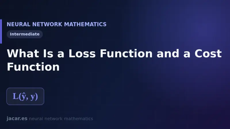
What Is a Loss Function and a Cost Function
A loss function measures how wrong a neural network is on a single example, comparing its prediction with the correct value. The cost function averages that loss across the whole dataset. That single number is exactly what training tries to reduce, step by step, using gradient descent to adjust every weight.
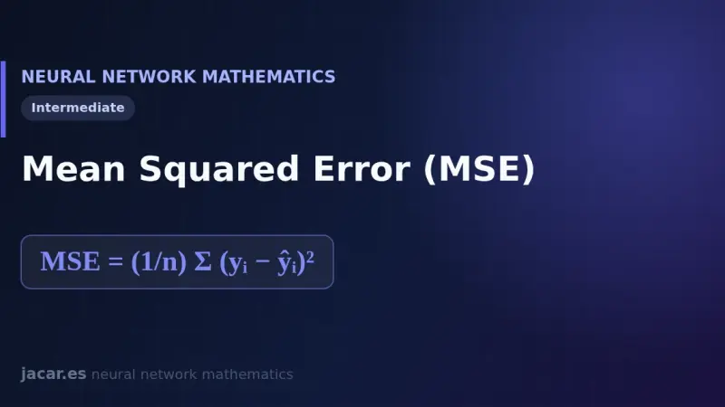
Mean Squared Error (MSE) as a Loss Function
Mean squared error (MSE) is the most common loss function in regression: it averages the square of the gap between each true value and its prediction. Squaring punishes big mistakes hard, keeps the function differentiable and gives gradient descent a clear, smooth target to minimise while training a model.
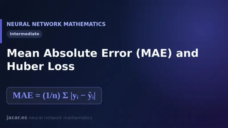
Mean Absolute Error (MAE) and Huber Loss
Mean absolute error (MAE) averages the absolute difference between prediction and reality, so a single outlier weighs only its fair share and never blows up the loss. Huber loss combines that robustness with the smoothness of mean squared error through a delta parameter that decides where the behaviour switches over.
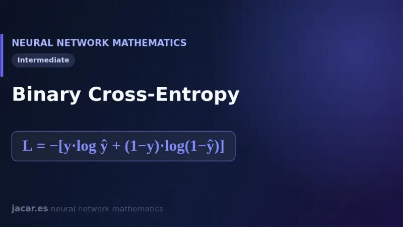
Binary Cross-Entropy
Binary cross-entropy is the standard loss function for two-class classification. It compares the probability returned by the sigmoid with the true label, 0 or 1, and punishes confident mistakes hard. Its formula comes from maximum likelihood, and its derivative combines with the sigmoid into a very simple gradient.
Categorical Cross-Entropy
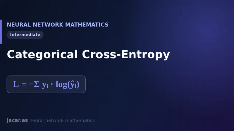
Categorical cross-entropy is the standard loss function for classifying into several mutually exclusive classes. It compares the distribution the network predicts, usually after a softmax, with the true label written in one-hot format, and it penalises heavily any low probability assigned to the correct class.
Entropy, Cross-Entropy and KL Divergence
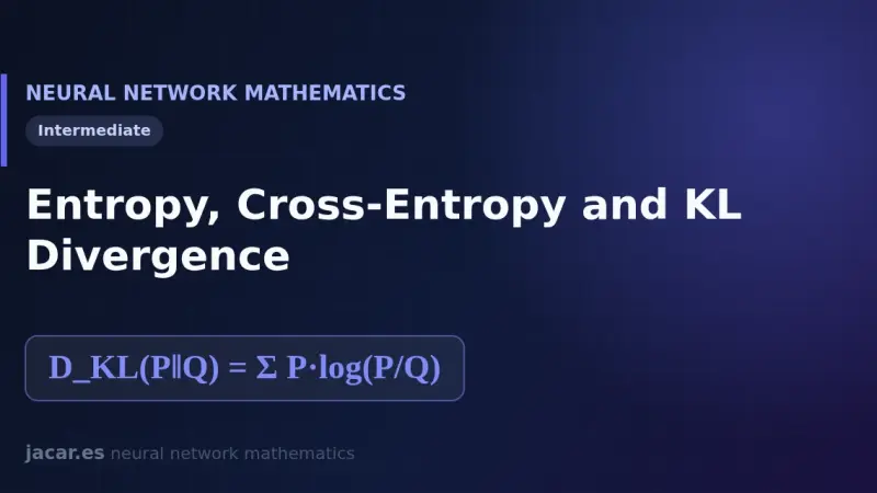
Entropy measures the average uncertainty of a distribution in bits, cross-entropy measures the cost of coding the real data with a wrong model, and KL divergence is the gap between the two. That is why minimising cross-entropy during training is the same as minimising the KL divergence from the labels.
L1 and L2 Regularization (Weight Decay)
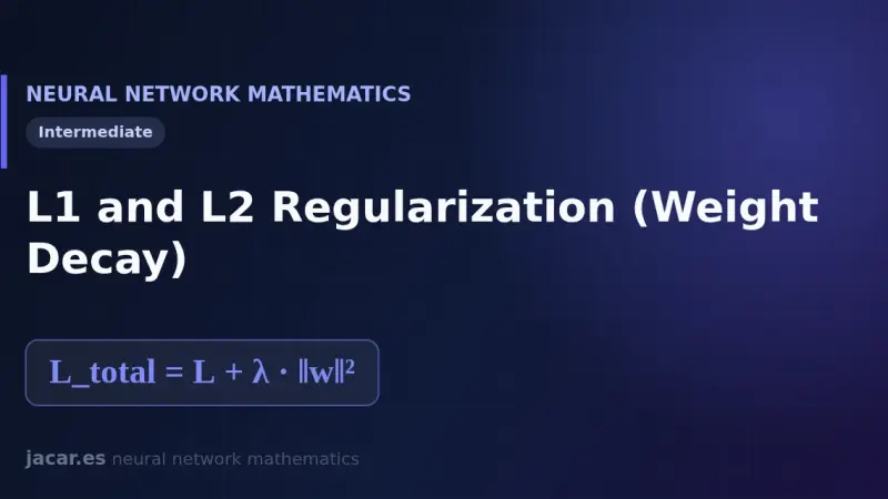
L1 and L2 regularization adds a term to the loss function that penalises large weights. L2, or weight decay, shrinks the weights smoothly towards zero; L1 drives them exactly to zero and yields sparse models. Both curb overfitting and improve the generalisation ability of a neural network on unseen data.