Categorical Cross-Entropy
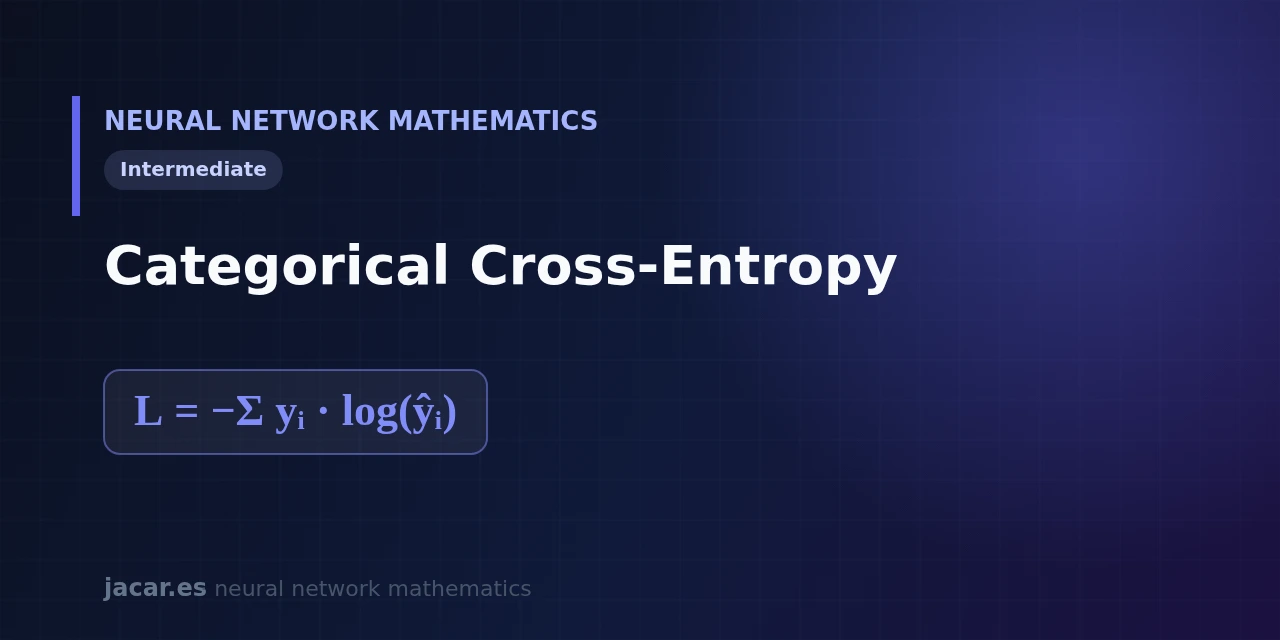
Table of contents
- Key takeaways
- What is categorical cross-entropy?
- Softmax and cross-entropy together
- Formula and one-hot encoding
- The simplified derivative (ŷ − y)
- A multi-class example
- Frequently asked questions
- How does it differ from binary cross-entropy?
- Should I pass it probabilities or logits?
- Why is the natural logarithm used?
- Conclusion
- Sources
Categorical cross-entropy is the loss function we use when a network must pick one class in a multi-class problem. It measures how far the probability distribution the model predicts sits from the correct answer, and it does so in a way that punishes confident mistakes hard. It is the natural partner of the softmax in the final layer of almost every modern classifier.
This guide walks through its formula, one-hot encoding and the derivative that makes it so convenient to train. The same explanation is available in Spanish.
Key takeaways
- Categorical cross-entropy is the default loss for classifying into three or more mutually exclusive classes.
- It compares two distributions: the predicted $\hat{y}$ (which sums to 1) and the true label $y$, written in one-hot format.
- Because only one component of $y$ equals 1, the loss reduces to $-\log(\hat{y}_c)$, where $c$ is the correct class.
- Combined with the softmax, its gradient simplifies to the subtraction $\hat{y}-y$, with no awkward derivatives in between.
- It is related to binary cross-entropy, which is the special two-class case.
What is categorical cross-entropy?
A multi-class classifier ends in a vector of probabilities. Faced with a photo it might say 0.7 that it is a cat, 0.2 that it is a dog and 0.1 that it is a bird. Those three numbers sum to 1 and form the prediction $\hat{y}$. The true label is another distribution, but a degenerate one: all the probability sits on the true class.
Cross-entropy measures the distance between those two distributions using ideas from Claude Shannon’s information theory. The more probability the model assigns to the correct class, the lower the loss; the more confidently it is wrong, the higher it grows. The idea is borrowed from statistics: minimising this loss is equivalent to maximum likelihood estimation. As Goodfellow, Bengio and Courville put it, «any loss consisting of a negative log-likelihood is a cross-entropy between the empirical distribution defined by the data and the model».
Softmax and cross-entropy together
Categorical cross-entropy almost never travels alone: it takes its input from a softmax function. The softmax takes the unnormalised scores of the final layer (the so-called logits) and turns them into positive probabilities that sum to 1. The loss then acts on that distribution.
This pairing is so common that libraries fuse it into a single operation for numerical stability. In PyTorch, torch.nn.CrossEntropyLoss internally applies log_softmax and the loss at once, so you pass it the raw logits, not probabilities. Merging both steps avoids computing exponentials and logarithms separately, where a large value could overflow in floating point.
Formula and one-hot encoding
The general formula for one example with $K$ classes is the one on the cover card:
$$L=-\sum_{i} y_i\log(\hat{y}_i)$$
Here $y_i$ is the true label of class $i$ and $\hat{y}_i$ the probability the model assigns to it. The label is written in one-hot format: a vector with a 1 in the position of the correct class and 0 everywhere else. With three classes, a cat would be $[1,0,0]$, a dog $[0,1,0]$ and a bird $[0,0,1]$.
One-hot encoding has a useful practical consequence. Because every term of the sum is multiplied by 0 except the one for the true class, the formula collapses to a single term:
$$L=-\log(\hat{y}_c)$$
In other words, the loss only looks at the probability the model gave to the correct answer. If it is right with $0.9$, the loss is about $0.105$; if it hesitates with $0.5$, it rises to $0.693$; and if it nearly rules it out with $0.1$, it shoots up to $2.303$. That logarithmic curve is what pushes the model to be confident when it is right.
Because the softmax never returns exactly 0, the logarithm is always defined. If the model assigned probability 0 to the correct class the loss would blow up to infinity. That is why you pass the raw logits and let the library fuse softmax and logarithm into one stable step.
The simplified derivative (ŷ − y)
The underlying reason softmax and cross-entropy always go hand in hand is their derivative. When training we need the gradient of the loss with respect to the logits z of the final layer. Derived separately, the softmax produces an awkward Jacobian matrix. But when you compose the two functions, almost everything cancels and a remarkably simple expression remains:
$$\frac{\partial L}{\partial z_i}=\hat{y}_i-y_i$$
The gradient is the prediction minus the true label. If the model predicts $0.7$ for the correct class when it should predict 1, the gradient in that component is $0.7-1=-0.3$, a direct signal of how much and in which direction to correct. This clean form makes backpropagation from the output layer cheap and stable, and it explains why this combination dominates classification.
Show the derivation
With the softmax $\hat{y}_i=\dfrac{e^{z_i}}{\sum_k e^{z_k}}$ and the loss $L=-\sum_k y_k\log\hat{y}_k$, the chain rule gives $\dfrac{\partial L}{\partial z_i}=\sum_k y_k(\hat{y}_i-\mathbf{1}[k=i])=\hat{y}_i\sum_k y_k-y_i$. Since the one-hot label satisfies $\sum_k y_k=1$, everything collapses to $\dfrac{\partial L}{\partial z_i}=\hat{y}_i-y_i$.
A multi-class example
Take a three-class classifier (cat, dog, bird) and an image whose true label is "cat", that is $y=[1,0,0]$. Suppose the softmax returns $\hat{y}=[0.7,\,0.2,\,0.1]$.
The loss is $-(1\cdot\log 0.7+0\cdot\log 0.2+0\cdot\log 0.1)=-\log 0.7\approx0.357$. Only the cat term counts. If in the next iteration the model improves and predicts $[0.9,\,0.05,\,0.05]$, the loss drops to $-\log 0.9\approx0.105$.
And the gradient with respect to the logits in the first case is $\hat{y}-y=[0.7-1,\,0.2,\,0.1]=[-0.3,\,0.2,\,0.1]$: it raises the logit of the correct class and pushes the other two down. With this loss as a compass, gradient descent tunes the weights iteration after iteration.
Frequently asked questions
How does it differ from binary cross-entropy?
The binary case has two classes and uses a single sigmoid output. The categorical one generalises to $K$ mutually exclusive classes with a softmax and a one-hot vector. When there are only two categories, both formulas give the same result.
Should I pass it probabilities or logits?
It depends on the library. In PyTorch, CrossEntropyLoss expects the raw logits because it applies the softmax internally; passing already-normalised probabilities would apply it twice. Read the documentation of the specific function before wiring it up.
Why is the natural logarithm used?
Because it links the loss to maximum likelihood and yields the clean derivative $\hat{y}-y$. The logarithm turns a product of probabilities into a manageable sum and penalises confident errors more and more steeply.
Conclusion
Categorical cross-entropy is the standard way of telling a classifier how wrong it is. Its formula looks dense, but with one-hot labels it reduces to looking at the probability of the correct class, and next to the softmax it hands you the cleanest possible gradient, the subtraction $\hat{y}-y$. The natural next step is to review how it fits into the full roadmap of the mathematics of neural networks.