The Computational Graph and Automatic Differentiation
Table of contents
- Key takeaways
- What is a computational graph
- Forward mode and reverse mode
- How automatic differentiation implements backpropagation
- Frameworks: PyTorch and TensorFlow
- A worked example of a graph
- Frequently asked questions
- How does automatic differentiation differ from symbolic and numerical differentiation?
- Why do neural networks use reverse mode and not forward mode?
- Do I need to understand the graph if I use PyTorch or TensorFlow?
- Conclusion
- Sources
Updated: 2026-10-19
A computational graph is the map of operations a neural network runs to turn its inputs into a loss, and automatic differentiation is the technique that walks that map to compute exact derivatives. Together they solve the central problem of training: knowing how to change each weight to reduce the error. This article explains what the graph is, how forward mode and reverse mode differ, and why backpropagation is just one concrete case of this machinery. The same explanation is available in Spanish.
Key takeaways
- A computational graph breaks a function into elementary operations (additions, products, activations) connected as nodes and edges.
- Automatic differentiation applies the chain rule over that graph to obtain exact derivatives, without the approximations of the numerical method.
- There are two modes: forward mode propagates derivatives ahead; reverse mode propagates them backward and is the one neural networks use.
- Reverse mode computes the gradient of every weight in a single backward pass, at a cost of only about 5 times that of evaluating the function.
- Backpropagation is automatic differentiation in reverse mode: PyTorch and TensorFlow build and run it for you.
What is a computational graph
When you write $L = (f(\mathbf{W}x+b)-y)^2$, that expression hides a sequence of simple operations. A computational graph makes them explicit: each node is an elementary operation (a matrix product, a bias addition, an activation, a subtraction) and each edge carries a value from one node to the next. Following the shared notation of this series, the weighted sum $z = \mathbf{W}x+b$ and the activation $a = f(z)$ are two chained nodes.
The advantage of this representation is twofold. First, computing the output means walking the graph from inputs to loss: that is forward propagation. Second, and more importantly, the structure of the graph holds all the information needed to differentiate.
Each node knows its local derivative with respect to its inputs, so it is enough to multiply and add those local derivatives along the graph’s paths. As chapter 6 of Deep Learning[1] sets out, this graph is the abstraction that turns gradient computation into a mechanical procedure.
Forward mode and reverse mode
Automatic differentiation can walk the graph in two directions. Forward mode propagates derivatives in the same order as the computation: it starts from an input and drags its derivative node by node to the output. Its cost is proportional to the number of inputs, so it is efficient when the outputs outnumber the inputs.
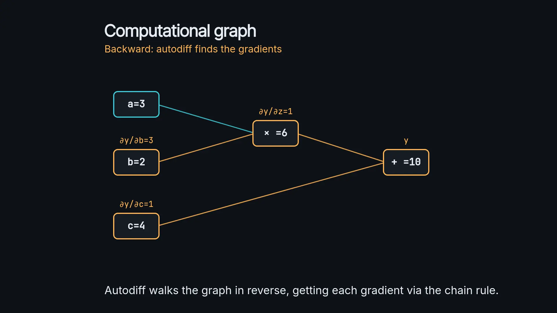
Reverse mode does the opposite. It first completes the forward pass, storing the intermediate values; then it walks the graph from the output back to the inputs, accumulating the derivative of the loss with respect to each node. Its cost is proportional to the number of outputs.
In a neural network the output is a single scalar (the loss $L$) and the inputs are millions of weights, so reverse mode obtains the full gradient $\nabla L$ in a single backward pass. A classic result, the Baur-Strassen theorem, guarantees that this gradient costs at most a constant factor (around 5) relative to evaluating the original function. That is why training a model with 175 billion parameters is still feasible: the gradient does not cost 175 billion times more than a prediction, only a few times more.
The price of reverse mode is memory: to differentiate it must keep every intermediate value from the forward pass until the backward pass finishes. That is why training consumes far more memory than merely predicting.
How automatic differentiation implements backpropagation
The backpropagation we studied in the chain rule is exactly reverse mode applied to a network’s graph. Each layer contributes its local derivative (that of the activation $f'(z)$, that of the product by $\mathbf{W}$, that of the bias) and reverse mode chains them from output to input. The chain rule thus shares out responsibility for the error $L$ layer by layer, without us having to write any derivative by hand.
This equivalence has history. Reverse mode was described by Seppo Linnainmaa in his 1970 master’s thesis; Paul Werbos connected it to neural networks in his 1974 doctoral thesis; and Rumelhart, Hinton and Williams popularised it in 1986. As Baydin and colleagues put it in their survey of the field, «backpropagation is a special case of reverse mode automatic differentiation». In other words, the hero formula of this article holds: reverse-mode autodiff is backpropagation.
Frameworks: PyTorch and TensorFlow
No engineer derives these expressions by hand. Frameworks build the graph for you and run reverse mode automatically.
PyTorch[2], available since 2017, uses an engine called autograd that builds the graph on the fly. Each operation on tensors that require gradients adds a node, and calling loss.backward() walks that graph backward and fills the .grad attribute of every parameter. This is known as a dynamic, define-by-run graph.
TensorFlow[3] follows a similar idea with tf.GradientTape: a context that records the operations executed so it can replay the backward pass afterwards. In both cases the pattern matches the theoretical graph: record operations forward, store the intermediate values and walk the record backward to obtain the gradients.
A worked example of a graph
This is the graph of a single neuron with a squared loss, with its forward pass and its backward pass:
Forward pass (from inputs to loss):
  x, W, b          input values
  z = W * x + b    operation 1: weighted sum
  a = f(z)         operation 2: activation
  L = (a - y)^2    operation 3: loss

Backward pass (chain rule, from L to the weights):
  dL/da = 2 * (a - y)
  dL/dz = dL/da * f'(z)
  dL/dW = dL/dz * x
  dL/db = dL/dz
Each line of the backward pass reuses the result of the previous one: that is the key to reverse mode’s efficiency. The derivative of the loss with respect to each weight is obtained without recomputing anything from the forward pass, because the intermediate values ($z$, $a$) were stored.
Show the derivation
Start from $L=(a-y)^2$ with $a=f(z)$ and $z=\mathbf{W}x+b$. The chain rule links the three local derivatives of the graph: $\dfrac{\partial L}{\partial \mathbf{W}} = \dfrac{\partial L}{\partial a}\cdot\dfrac{\partial a}{\partial z}\cdot\dfrac{\partial z}{\partial \mathbf{W}} = 2(a-y)\cdot f'(z)\cdot x$. Each factor is exactly one of the nodes in the backward pass: $2(a-y)$ is $\partial L/\partial a$, $f'(z)$ maps from $a$ to $z$ and $x$ maps from $z$ to $\mathbf{W}$.
Frequently asked questions
How does automatic differentiation differ from symbolic and numerical differentiation?
Numerical differentiation approximates the derivative with small perturbations and carries rounding errors. Symbolic differentiation manipulates formulas and can grow explosively. Automatic differentiation evaluates exact derivatives operation by operation at a controlled cost: it combines the precision of the symbolic approach with the efficiency of the numerical one.
Why do neural networks use reverse mode and not forward mode?
Because a network has one output (the loss) and millions of inputs (the weights). Reverse mode’s cost depends on the number of outputs, so with a single output it computes the gradient of every weight in one pass. Forward mode would need one pass per weight.
Do I need to understand the graph if I use PyTorch or TensorFlow?
For simple tasks, the framework handles it for you. But understanding the graph helps you debug gradients that do not flow, manage memory (intermediate values take up space) and know when to disconnect parts of the graph with operations such as detach().
Conclusion
The computational graph and automatic differentiation are the quiet infrastructure of deep learning: they turn an arbitrary function into a network of differentiable operations and compute its gradient exactly and cheaply. Reverse mode, with its single backward pass, is what makes training scalable. The natural next step is to review how those derivatives chain together in the chain rule and to return to the general mathematics roadmap to place each piece.
Sources: [1] Autograd (PyTorch documentation)[2], [2] Introduction to gradients and automatic differentiation (TensorFlow)[3], [3] Deep Learning (Goodfellow, Bengio and Courville)[1], [4] Automatic differentiation in machine learning: a survey (Baydin et al.)[4], [5] Automatic differentiation (Wikipedia)[5].