pgvector: Semantic Search Without Leaving Postgres

Tested with PostgreSQL 18.6 · pgvector 0.8.6 · Docker · verified 2026-09-16

Updated: 2026-09-16

Semantic search (retrieving documents by meaning rather than keyword match) has quietly become the foundation of much of the LLM application boom. Behind every RAG system, every assistant that consults internal documentation, every "smart" search bar, sits the same mechanic. A model turns text into a vector of hundreds or thousands of dimensions, and the application looks for vectors close to the query.

What is interesting is that setting that up does not require introducing a brand new database into the stack, provided you already run PostgreSQL. pgvector^[1] turns an existing PostgreSQL into a perfectly competent vector database. This text was revised on 16 September 2026 for pgvector 0.8.6 and PostgreSQL 18.6, with figures measured on 99,000 real embeddings. To install it, follow the step-by-step PostgreSQL with pgvector guide.

Key takeaways

• pgvector extends PostgreSQL with the vector type (and, since 0.7.0, with halfvec, sparsevec and bit indexing) plus cosine, Euclidean, inner-product and L1 distance operators.

• It has two approximate nearest-neighbour (ANN) indexes: HNSW, a layered graph with a better recall-latency trade-off, and IVFFlat, which clusters vectors with k-means and builds faster.

• On 99,000 embeddings with 1,536 dimensions, HNSW with its defaults reached 95.1% recall@10 at a 1.15 ms median; exact search took 158.9 ms.

• With an approximate index, the WHERE clause is applied after the index scan: a selective condition returns fewer rows than requested unless you enable the iterative index scans added in 0.8.0.

• That test’s HNSW index takes 773 MB, about 7.6 GB per million vectors. When it no longer fits in RAM, try halfvec or binary quantisation before switching databases.

Why semantic search needs a different kind of index

A modern embedding (think of the 1,536 values OpenAI’s text-embedding-3-small produces by default) lives in a high-dimensional space. Finding the vector most similar to another is, mathematically, computing a distance (cosine, Euclidean, or inner product) against every stored vector. In this article’s test, that exact search over 99,000 documents took a 158.9 ms median. With ten million, the linear estimate is around 16 s, and the user has already left.

Postgres’s classic B-tree indexes, designed to order scalars, do not work for vectors. A B-tree needs a total order; in a 1,536-dimensional space that order does not exist. The industry’s practical answer has been to give up exactness and accept approximate search, ANN (approximate nearest neighbour). In the same test, HNSW answered in a 1.15 ms median, about 138 times less than exact search, at the cost of 4.9 points of recall@10.

pgvector implements this idea with two index types. HNSW builds a multilayer graph and, according to the project documentation, offers a better speed-recall trade-off than IVFFlat, at the cost of slower builds and more memory. IVFFlat partitions the table into lists with k-means at build time, and each query compares only against vectors in the lists nearest the query point. The hnsw.ef_search (40 by default) and ivfflat.probes (1 by default) parameters are tunable per query: raising them improves recall and adds latency.

When pgvector is the right call

The honest question is not "is pgvector the best?" but "what does my project actually gain by using Qdrant, Pinecone, or Milvus instead of extending the Postgres it already has?". The answer tends to be: less than it looks.

You already have backups, monitoring, replication, and an access policy working on Postgres. Adding a separate vector service doubles that surface: another process to patch, another backup to test, another maintenance window to coordinate.

There is also an architectural advantage that gets systematically underrated. In a dedicated vector database, metadata (author, category, date, permissions) lives in a different part of the system. Any complex filter requires coordinating two stores.

With pgvector, WHERE category = 'tech' AND user_id = 42 and the vector ranking live in the same query and the Postgres planner decides how to execute them together. That single fact eliminates an entire layer of glue code.

Even so, pgvector is not the universal answer. The vector type stores up to 16,000 dimensions, but its indexes stop at 2,000. Because text-embedding-3-large returns 3,072 by default, you would have to index it as halfvec (up to 4,000), with binary quantisation, or by asking the model for fewer dimensions.

The other limit is memory, because an index that does not fit in RAM forces disk reads on every query. For internal chatbots, documentation assistants and support search, with tens or hundreds of thousands of chunks, those limits are a long way away.

From CREATE EXTENSION to an index that performs

Getting started takes three statements, and the index is best created after the initial load:

CREATE EXTENSION IF NOT EXISTS vector;

CREATE TABLE documents (
    id        bigserial PRIMARY KEY,
    content   text,
    category  text,
    embedding vector(1536)  -- text-embedding-3-small
);

-- After the initial load
CREATE INDEX CONCURRENTLY documents_embedding_idx
    ON documents USING hnsw (embedding vector_cosine_ops);

-- IVFFlat alternative for one million rows: lists = rows / 1000
-- CREATE INDEX CONCURRENTLY documents_embedding_ivf
--     ON documents USING ivfflat (embedding vector_cosine_ops)
--     WITH (lists = 1000);

HNSW can be created on an empty table because it has no training step, but the pgvector documentation recommends creating any index after loading the data, because it builds faster. IVFFlat does need data: it computes its lists from the vectors it finds at build time. CONCURRENTLY avoids blocking writes in the meantime.

The query combines the relational filter with the distance ordering. $1 is the question’s embedding, which your application passes as a parameter:

SET hnsw.ef_search = 100;
SET hnsw.iterative_scan = strict_order;

SELECT id, content, 1 - (embedding <=> $1::vector) AS score
FROM documents
WHERE category = 'tech'
ORDER BY embedding <=> $1::vector
LIMIT 5;

I ran it as written, through PREPARE, on 20,000 real rows spread over five categories, and it returned the 5 requested rows. With the index forced, iterative scans off and hnsw.ef_search = 10, the same query returned only 2. The next section explains why.

These are the distance operators in pgvector 0.8.6:

• <=>: cosine distance, the usual one for semantic search

• <->: Euclidean (L2) distance

• <#>: negative inner product

• <+>: L1 distance, since 0.7.0

• <~> and <%>: Hamming and Jaccard distances for binary (bit) vectors

Cosine similarity comes out as 1 - (a <=> b): it is 1 when the vectors point the same way and 0 when they are orthogonal. OpenAI normalises its embeddings to length 1, so cosine, inner product and Euclidean distance rank them identically. That is why the pgvector documentation recommends <#> for exact search, which saves computation. If you use an index, build it with the operator class of the distance you query (vector_ip_ops for <#>).

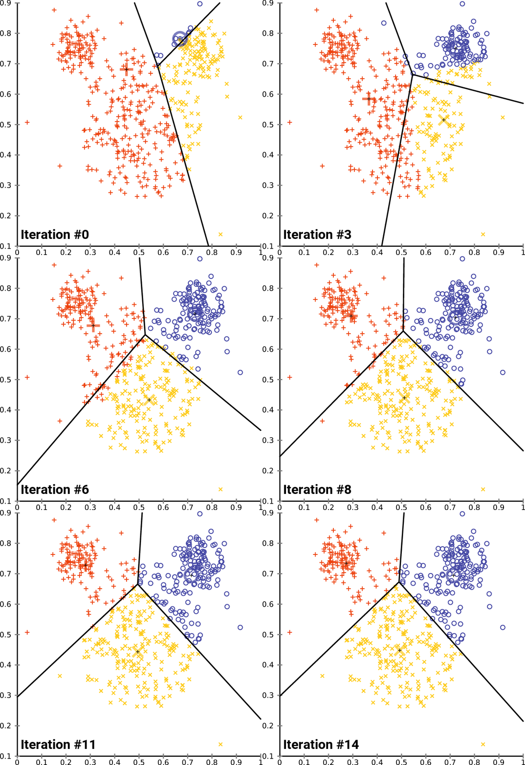Animation of k-means converging, the algorithm IVFFlat uses to partition vectors into lists when it builds the index (Image: Chire, CC BY-SA 4.0, via Wikimedia Commons)

Three operational details that make the difference

• Build the index with CREATE INDEX CONCURRENTLY to avoid blocking writes during the operation, as the pgvector documentation recommends for production. If PostgreSQL runs in Docker and the build is parallel, give the container a --shm-size at least as large as maintenance_work_mem. With the 64 MB default, my parallel HNSW build failed with No space left on device.

• Measure recall instead of reindexing on a calendar: IVFFlat fixes its lists at build time, and if new vectors drift away from the original distribution, recall drops. Compare the index results with exact search from time to time (SET LOCAL enable_indexscan = off inside a transaction) and rebuild with REINDEX INDEX CONCURRENTLY when it falls. With HNSW, run at least 0.8.4: 0.8.3 and 0.8.4 fixed possible index corruption and the “hnsw graph not repaired” error during VACUUM.

• Treat filters for what they are: with an approximate index, PostgreSQL scans the index and filters afterwards. In a test with 20,000 rows, a filter matching 10% of them with hnsw.ef_search = 40 returned 4 of the 10 requested rows; with hnsw.iterative_scan = relaxed_order it returned all 10. Without forcing the index, the 0.8.6 planner chose an exact sequential scan there, and 0.8.0 had already improved that cost estimation. If the filter leaves few rows, add a B-tree index on the column so the exact search over that subset does not scan the whole table.

For IVFFlat, the pgvector documentation suggests lists = rows / 1000 up to one million rows, sqrt(rows) above that, and starting with probes = sqrt(lists). I measured it on 99,000 text-embedding-3-small embeddings from the DBpedia dataset Qdrant publishes on Hugging Face^[2], with 1,000 held-out queries from the same dataset and the exact top 10 as ground truth:

The figures come from PostgreSQL 18.6 with pgvector 0.8.6 in the pgvector/pgvector:0.8.6-pg18-trixie image. The 18-core arm64 machine was shared with other processes, with a load average between 3.5 and 6.6 during the run. To isolate each index I forced it with enable_seqscan = off, because at ef_search = 100 the planner picked exact search for the sample query. Building the HNSW index took 23.0 s with four parallel workers, and the IVFFlat one 4.3 s; both take about 773 MB.

The practical conclusion is that HNSW with its defaults already beats IVFFlat with 10 probes on both recall and latency. IVFFlat pays off when build time is what matters, and even then probes = sqrt(lists) (10 probes for 100 lists) stopped at 92.8%.

Signs you have outgrown pgvector

There are clear symptoms that a project has grown past what the extension comfortably covers:

• Sustained p95 latency above 100 ms with parameters properly tuned.

• Indexes that no longer fit in RAM and force disk reads on every query.

• You already use halfvec or binary quantisation with re-ranking (both available since 0.7.0) and the index still does not fit in memory.

Before migrating, the pgvector documentation suggests scaling vertically, adding read replicas or sharding with Citus. If none of that is enough, Qdrant is the pragmatic next step: it keeps the self-hostable property and scales much better. But getting there is itself a sign of success, not an architectural failure: it means the project works well enough to stress the infrastructure.

If you use LangChain or Chroma for the RAG pipeline, migrating the retriever from pgvector to Qdrant is a few-line change, as long as you respected the retriever abstraction from the start.

Conclusion

pgvector is not the fastest link on the market and does not pretend to be. It is the piece that lets you add semantic search to an existing product without multiplying the operational surface, reusing the Postgres your team already knows how to operate, back up, and audit. With RAG becoming the default pattern, that combination of pragmatism and conservative engineering is what separates the prototypes that reach production from the ones that stay as demos.

Frequently asked questions

How should I set the lists and probes parameters for a pgvector IVFFlat index?

Start where the pgvector documentation does: lists at rows / 1000 up to one million rows and at the square root of the row count above that, and ivfflat.probes at the square root of lists. On 99,000 embeddings with 1,536 dimensions and 100 lists, 10 probes gave 92.8% recall@10 and 20 probes 96.8%, at 8.7 and 14.9 ms medians. Build the index after loading representative data, because the lists are computed at that moment, and use CREATE INDEX CONCURRENTLY if the table takes writes.

Can I combine a normal SQL WHERE filter with vector similarity ranking in pgvector?

Yes, in the same SQL query, with one caveat: with an approximate index, PostgreSQL filters after scanning the index. With a filter matching 10% of the rows and hnsw.ef_search = 40, the query returned 4 of the 10 requested rows. Since 0.8.0, hnsw.iterative_scan (strict_order or relaxed_order) and ivfflat.iterative_scan = relaxed_order keep scanning until enough rows are found, and with relaxed_order the query returned all 10. For filters that leave few rows, a B-tree index on the column allows an exact search over that subset.

When have I outgrown pgvector and should move to Qdrant or Pinecone?

When measurable signals say so: p95 latency above 100 ms with tuned parameters, indexes that no longer fit in RAM, or memory that runs short even with halfvec and binary quantisation. For scale, the HNSW index for 99,000 vectors with 1,536 dimensions took 773 MB, about 7.6 GB per million. Before migrating, try scaling vertically, adding replicas or sharding with Citus. If that is not enough, Qdrant is the pragmatic next step, and with LangChain the retriever swap is a few-line change.

Should I use HNSW or IVFFlat in pgvector?

Start with HNSW and its defaults (m = 16, ef_construction = 64). In this article’s test it reached 95.1% recall@10 at a 1.15 ms median, against 92.8% and 8.7 ms for IVFFlat with 100 lists and 10 probes. IVFFlat builds faster (4.3 s against 23.0 s with four parallel workers) and needs data before it can be created, so it makes sense when the maintenance window is short.

Sources

1. pgvector
2. DBpedia dataset Qdrant publishes on Hugging Face
3. pgvector: Changelog
4. PostgreSQL: CREATE INDEX CONCURRENTLY documentation
5. OpenAI: Embeddings guide and text models