The Fully Connected Neural Network: An Innovative Approach to Machine Learning

In a fully connected neural network, each neuron in a layer is linked to every neuron in the previous and next layer. This total connectivity makes it the most expressive architecture and also the most computationally costly: it is the mandatory starting point for understanding deep learning.

Key takeaways

• Each neuron receives the output of every neuron in the preceding layer, multiplied by a learnable weight.

• The architecture can model complex non-linear relationships between inputs and outputs.

• Power increases with depth, but so does the risk of overfitting and computational cost.

• In vision, they are combined with convolutional layers; in NLP, with attention mechanisms.

• The choice of activation function (ReLU, sigmoid, tanh) determines the capacity to learn non-linear relationships.

Architecture: how layers connect

A fully connected network is organised into three types of layers:

• Input layer: receives raw data (pixels, tabular values, embeddings).

• Hidden layers: successively transform the representation; each neuron applies an activation function to its weighted input sum.

• Output layer: produces the final prediction, a continuous value for regression or a probability for classification.

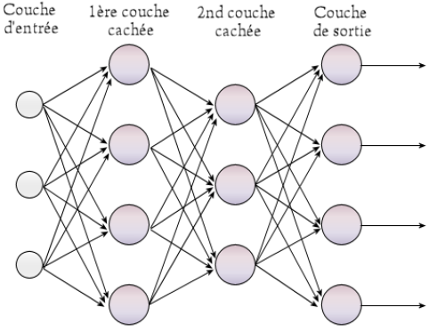
The number of parameters (weights) grows quadratically with the number of neurons: a layer of 1,000 neurons connected to another of 1,000 has 10⁶ weights. This makes dense networks infeasible for high-resolution images without specialised architectures like convolutional ones.

Forward propagation and training

The data flow in a dense network:

• Inputs are multiplied by layer 1 weights and summed (dot product).

• The activation function is applied: ReLU, tanh, sigmoid, depending on the architecture.

• Output passes to the next layer and the process repeats.

• At the final layer, the loss function compares the prediction to the true label.

• The loss gradient is propagated backwards (backpropagation), adjusting all weights.

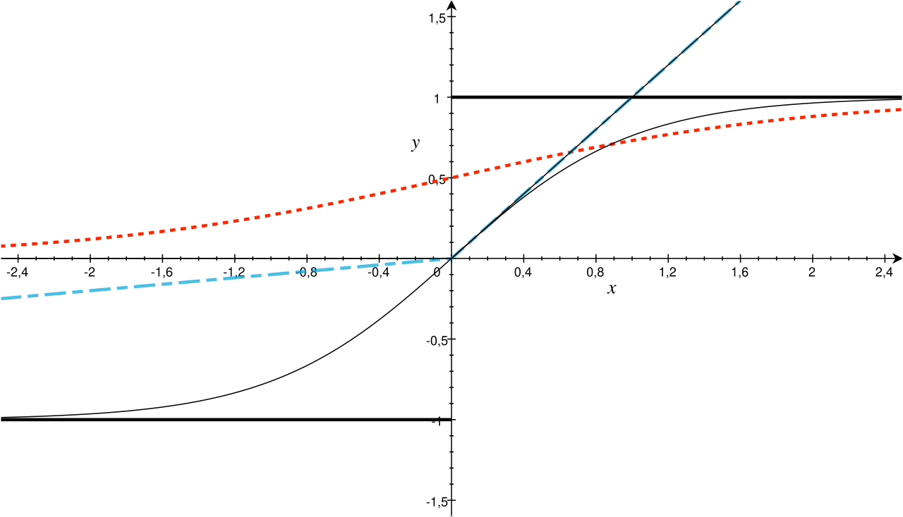Comparison of activation functions used in the layers of a dense network (Image: Andreas Maier, CC BY 4.0, via Wikimedia Commons)

Main applications

Fully connected networks work well for:

• Tabular data classification: churn prediction, credit scoring, fraud detection.

• Pattern recognition: combined with feature extraction layers (CNN for images, RNN for sequences).

• Time series prediction: with LSTM + dense layer architectures at the output.

• Natural language processing: as a classification head over pre-trained embeddings.

Advantages and limitations

Advantages:

• Universal approximation capacity: with sufficient depth and width, it can model any continuous function (universal approximation theorem).

• Versatility: works with any vectorised input type.

• Ease of interpretation at the output layer.

Limitations:

• Quadratic computational cost in the number of neurons.

• Prone to overfitting on small datasets: requires regularisation (dropout, L2).

• Does not incorporate translation or permutation invariance: for images, CNNs are more efficient; for sequences, RNNs or transformers.

Conclusion

The fully connected neural network is the fundamental building block of deep learning: the conceptual and practical starting point for any more specialised architecture. Understanding how information flows through dense layers, what role each activation function plays, and how gradients adjust weights is the foundation on which CNNs, RNNs, transformers, and everything that has followed are built. Mastering it is non-negotiable for anyone who wants to work with applied AI.

Frequently asked questions

Why can't I just use a fully connected network on high-resolution images?

Because the number of weights grows quadratically with the number of neurons. A layer of 1,000 neurons connected to another of 1,000 already has 10⁶ weights, which makes dense networks infeasible for high-resolution images without specialised architectures. Dense layers also lack translation invariance, so for images convolutional layers are more efficient and the fully connected part is left with one role: a classification head on top of the extracted features.

How do I stop a fully connected network from overfitting on a small dataset?

Apply regularisation, such as dropout or L2, because dense networks are prone to overfitting when data is scarce. Keep in mind that power increases with depth and width, but so do the overfitting risk and the computational cost, so adding layers is not a free win. The universal approximation theorem says a sufficiently deep and wide network can model any continuous function, which is exactly why it will also fit noise if you let it.