Gradients of a Dense Layer: Matrices and Jacobians
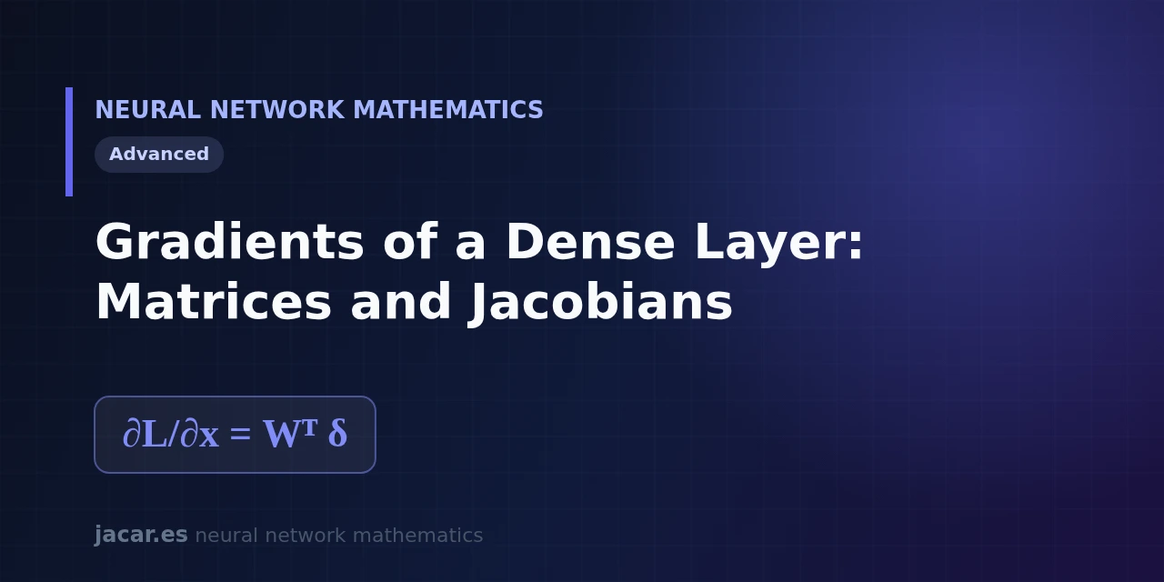
Table of contents
- Key takeaways
- The Jacobian matrix
- Gradient with respect to the weights
- Gradient with respect to the input
- Why the transpose of W appears
- Example with dimensions
- Frequently asked questions
- What exactly is the Jacobian of a dense layer?
- Why is the weight gradient an outer product?
- How do I check that I am not getting the transposes wrong?
- Conclusion
- Sources
The gradient of a dense layer reduces to two formulas, and both are born from a single Jacobian matrix. When a layer computes $\mathbf{z} = \mathbf{W}\mathbf{x}+\mathbf{b}$, the derivative of the output with respect to the input is not a lone number but a full matrix: the Jacobian. Understanding that matrix explains why the gradient with respect to the weights is $\boldsymbol{\delta}\,\mathbf{x}^\top$ and why the one travelling backward is $\mathbf{W}^\top \boldsymbol{\delta}$.
This guide derives both results with concrete dimensions. The same explanation is available in Spanish.
Key takeaways
- The Jacobian of a vector function collects every partial derivative of each output with respect to each input in a single matrix.
- For a dense layer $\mathbf{z} = \mathbf{W}\mathbf{x}+\mathbf{b}$, the Jacobian of $\mathbf{z}$ with respect to $\mathbf{x}$ is exactly the weight matrix $\mathbf{W}$.
- The gradient of the loss with respect to the weights is an outer product: $\frac{\partial L}{\partial \mathbf{W}} = \boldsymbol{\delta}\,\mathbf{x}^\top$, with the same dimensions as $\mathbf{W}$.
- The gradient with respect to the input is $\frac{\partial L}{\partial \mathbf{x}} = \mathbf{W}^\top \boldsymbol{\delta}$, and that transpose is what propagates the error to the previous layer.
- If $\mathbf{W}$ is $3 \times 4$, the gradient $\boldsymbol{\delta}\,\mathbf{x}^\top$ is also $3 \times 4$ and $\mathbf{W}^\top \boldsymbol{\delta}$ has 4 components: the dimensions match or something is wrong.
The Jacobian matrix
When a function takes a vector and returns another vector, its derivative stops being a number and becomes a matrix. That matrix is the Jacobian. If a function maps an input of $n$ components to an output of $m$ components, its Jacobian is a table of $m \times n$ numbers, where row $i$ and column $j$ hold the partial derivative of output $i$ with respect to input $j$.
It is the natural extension of the partial derivative and the gradient: instead of a single output, we have a whole vector of them, and each component contributes its own row of partials. Wikipedia[1] puts it precisely: the Jacobian is the best linear approximation of the function near a point. As Terence Parr and Jeremy Howard write in their essay on matrix calculus, «this paper is an attempt to explain all the matrix calculus you need in order to understand the training of deep neural networks».
The Jacobian of the linear part is constant: it equals $\mathbf{W}$ whatever the value of $\mathbf{x}$. That sets it apart from the Jacobian of an activation such as the sigmoid, which does change with the input.
Gradient with respect to the weights
To train, we need to know how the loss $L$ changes as we move each weight. We first define the layer error, $\boldsymbol{\delta} = \frac{\partial L}{\partial \mathbf{z}}$, a vector with as many components as $\mathbf{z}$ has outputs. That $\boldsymbol{\delta}$ arrives from the later layers through the chain rule.
Because $\mathbf{z} = \mathbf{W}\mathbf{x}+\mathbf{b}$, each output $zi$ depends on the weight $W{ij}$ in a simple way: $\frac{\partial zi}{\partial W{ij}} = x_j$. Applying the chain rule and arranging the terms, the full gradient is an outer product:
$$\frac{\partial L}{\partial \mathbf{W}} = \boldsymbol{\delta}\,\mathbf{x}^\top$$
Here $\boldsymbol{\delta}$ is a column vector and $\mathbf{x}^\top$ a row vector, so their product rebuilds a matrix with the exact shape of $\mathbf{W}$. Each entry says how much that weight contributes to the error, combining the signal coming in through $\mathbf{x}$ with the error going out through $\boldsymbol{\delta}$.
Gradient with respect to the input
The second gradient does not tune this layer but shares the blame backward. We want $\frac{\partial L}{\partial \mathbf{x}}$, that is, how much the loss would have changed had the input been different. That value is the $\boldsymbol{\delta}$ of the previous layer.
We start from the Jacobian of $\mathbf{z}$ with respect to $\mathbf{x}$. Since $\mathbf{z} = \mathbf{W}\mathbf{x}+\mathbf{b}$, the partial $\frac{\partial z_i}{\partial xj}$ is $W{ij}$, so the full Jacobian is the matrix $\mathbf{W}$ itself. Chaining that Jacobian with the error $\boldsymbol{\delta}$, the chain rule for vectors multiplies by the transpose:
$$\frac{\partial L}{\partial \mathbf{x}} = \mathbf{W}^\top \boldsymbol{\delta}$$
This is the central result of the article, and also the formula on the cover image. The same matrix multiplication we studied in matrix multiplication in neural networks reappears here, now in the backward pass.
Show the derivation
By the chain rule, $\frac{\partial L}{\partial x_j} = \sum_i \frac{\partial L}{\partial z_i}\,\frac{\partial z_i}{\partial x_j} = \sum_i \delta_i\,W_{ij}$. That sum over $i$ runs down column $j$ of $\mathbf{W}$, which is row $j$ of $\mathbf{W}^\top$; gathering the $n$ components into a vector gives the matrix form $\frac{\partial L}{\partial \mathbf{x}} = \mathbf{W}^\top \boldsymbol{\delta}$.
Why the transpose of W appears
The natural question is why the forward pass uses $\mathbf{W}$ and the backward pass $\mathbf{W}^\top$. The reason is purely dimensional and about orientation. In forward propagation, $\mathbf{W}$ takes an input vector of $n$ components and produces $m$ outputs. In backpropagation we walk the reverse path: we start from an error with $m$ components and must return a vector with $n$ components, one per input.
Only an $n \times m$ matrix can turn $m$ numbers into $n$, and that matrix is $\mathbf{W}^\top$. Put another way, the transpose swaps the roles of rows and columns exactly as needed for the error to flow the other way. It is not a trick: it is what the chain rule demands when the layer’s Jacobian is $\mathbf{W}$. This same mechanism is the heart of the step-by-step derivation of backpropagation.
Example with dimensions
Let us put in concrete numbers. Suppose a layer with $n = 4$ inputs and $m = 3$ outputs. Then $\mathbf{W}$ is a $3 \times 4$ matrix, with 12 weights, the vector $\mathbf{x}$ has 4 components and $\mathbf{z}$ has 3. The bias $\mathbf{b}$ adds another 3 values.
In the backward pass, the error $\boldsymbol{\delta}$ has 3 components, one per output. Let us check the two formulas:
- $\frac{\partial L}{\partial \mathbf{W}} = \boldsymbol{\delta}\,\mathbf{x}^\top$: a vector of 3 times a row vector of 4 gives a $3 \times 4$ matrix, identical to $\mathbf{W}$. Correct.
- $\frac{\partial L}{\partial \mathbf{x}} = \mathbf{W}^\top \boldsymbol{\delta}$: the transpose $\mathbf{W}^\top$ is $4 \times 3$, and multiplying by $\boldsymbol{\delta}$ of 3 components yields a vector of 4, one per input. Correct.
Matching the dimensions is the best quick check: if at any step the shapes do not fit, there is a transpose or an ordering error in the product. With learning rate $\eta$, the final update is $\mathbf{W} \leftarrow \mathbf{W}-\eta\,\frac{\partial L}{\partial \mathbf{W}}$, one step of gradient descent applied to all 12 components at once.
Frequently asked questions
What exactly is the Jacobian of a dense layer?
It is the matrix of all partial derivatives of the output with respect to the input. For $\mathbf{z} = \mathbf{W}\mathbf{x}+\mathbf{b}$, that Jacobian is the weight matrix $\mathbf{W}$, because each $\frac{\partial z_i}{\partial xj}$ equals precisely $W{ij}$. That is why the linear part of the layer has a constant Jacobian that does not depend on the value of $\mathbf{x}$.
Why is the weight gradient an outer product?
Because it combines two vectors of opposite directions: the error $\boldsymbol{\delta}$ coming down from the later layers and the input $\mathbf{x}$ that went up in the forward pass. The product $\boldsymbol{\delta}\,\mathbf{x}^\top$ crosses each component of the error with each component of the input, and the result has exactly the shape of $\mathbf{W}$, so it can be subtracted weight by weight.
How do I check that I am not getting the transposes wrong?
By verifying the dimensions at every step. If $\mathbf{W}$ is $3 \times 4$, then $\mathbf{W}^\top \boldsymbol{\delta}$ must give a vector of 4 and $\boldsymbol{\delta}\,\mathbf{x}^\top$ a $3 \times 4$ matrix. When the shapes do not match, there is almost always a missing transpose or the product is in the wrong order.
Conclusion
The gradient of a dense layer rests on a single idea: the Jacobian of $\mathbf{z} = \mathbf{W}\mathbf{x}+\mathbf{b}$ with respect to the input is the matrix $\mathbf{W}$. From it the two formulas that drive training follow, $\frac{\partial L}{\partial \mathbf{W}} = \boldsymbol{\delta}\,\mathbf{x}^\top$ to adjust the weights and $\frac{\partial L}{\partial \mathbf{x}} = \mathbf{W}^\top \boldsymbol{\delta}$ to propagate the error. The natural next step is to see these pieces chained together inside the roadmap of the mathematics of neural networks.
Sources: [1] Deep Learning (Goodfellow, Bengio and Courville)[2], [2] The Matrix Calculus You Need For Deep Learning (Parr and Howard)[3], [3] Jacobian matrix and determinant (Wikipedia)[1], [4] Backpropagation through a fully-connected layer (Eli Bendersky)[4].