A healthcheck is a command Docker runs periodically inside the container to decide whether the service is healthy; its state moves from starting to healthy or unhealthy. Combined with a restart policy (no, always, on-failure or unless-stopped) and with depends_on and the service_healthy condition, it stops an application from starting before its database.
Docker Compose gives you three ways to pass configuration into a container: the environment key, the env_file attribute and the .env file for interpolation. For sensitive data, do not use environment variables; Docker Compose secrets are mounted as read-only files under /run/secrets/, away from logs and the process environment.
A container loses its data the moment you delete it, unless you store that data outside. Docker gives you two ways: named volumes, which it manages itself under /var/lib/docker/volumes, and bind mounts, which link a host folder. Here you will see when to use each, how to mount them in Compose and how to back them up.
Docker ships six network drivers: bridge, host, none, overlay, macvlan and ipvlan. The default bridge network connects containers by IP but without name resolution. A user-defined bridge adds an internal DNS server so services find each other by name, and it is the recommended choice for almost any deployment.
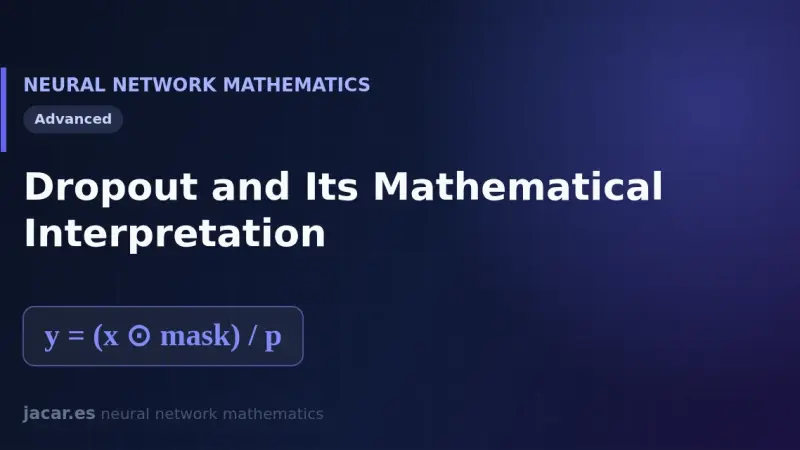
Dropout is a regularization technique that switches neurons off at random during training, with retention probability p, and divides the surviving activations by p to preserve their scale. At inference the full network runs without dropping anything. Mathematically it amounts to averaging a huge ensemble of subnetworks that share weights.
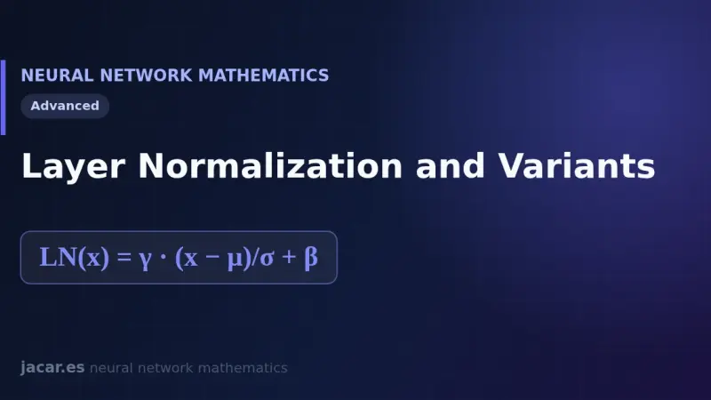
Layer normalization stabilizes training by normalizing each example on its own, using the mean and standard deviation of its own activations. Unlike batch normalization, it does not depend on the batch size, which is why transformers adopted it. RMSNorm is its lighter, most widely used variant today in large language models.
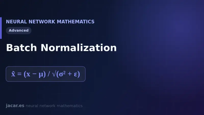
Batch normalization is a technique that normalises each layer's activations using the mean and variance of the mini-batch, then rescales them with two learnable parameters, gamma and beta. Introduced in 2015, it enables higher learning rates, speeds up training and stabilises deep neural networks during optimisation.
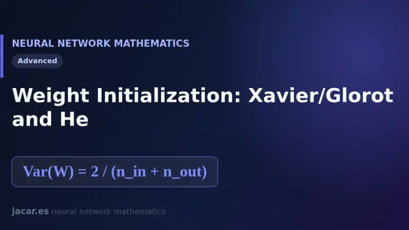
Weight initialization sets the starting scale of the matrix W before training begins. Xavier/Glorot, from 2010, splits the variance between inputs and outputs and suits sigmoid and tanh; He, from 2015, doubles it for ReLU, which zeroes half the activations. A poor choice stalls or breaks learning.
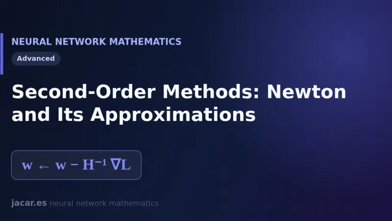
Second-order methods use the Hessian, the matrix of second derivatives of the loss, to orient each step better than the gradient alone. Newton's method updates the weights by subtracting the inverse Hessian times the gradient, but inverting it is far too costly in large networks, so practitioners fall back on quasi-Newton approximations.
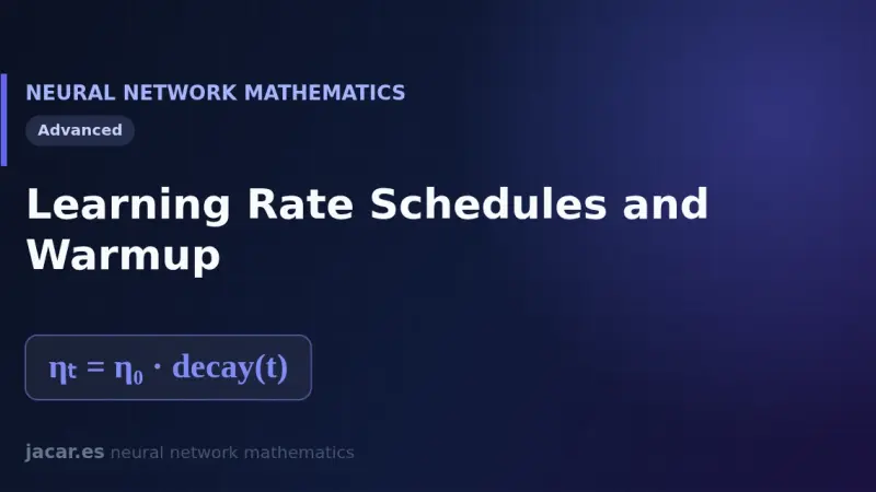
A learning rate schedule changes the value of η over the course of training instead of keeping it fixed. It starts with a warmup that raises η from near zero, holds a peak and then lowers it with step, exponential or cosine decay so the network converges faster and with far less oscillation.
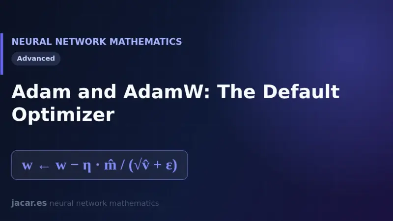
Adam combines a first-order moment (a moving average of the gradient) and a second-order moment (an average of its squares) to give each parameter its own learning rate. With bias correction and the defaults β1=0.9, β2=0.999 and ε=1e-8, it converges fast with almost no tuning.
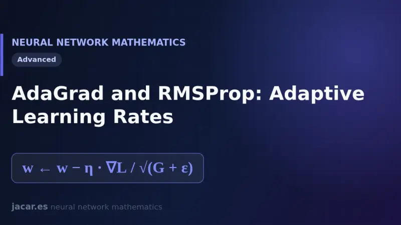
AdaGrad and RMSProp are optimisers that give every weight its own learning rate. AdaGrad accumulates the square of all past gradients and divides the step by its root, which slowly fades it out. RMSProp fixes this with a moving average that forgets the past using a decay factor of about 0.9.
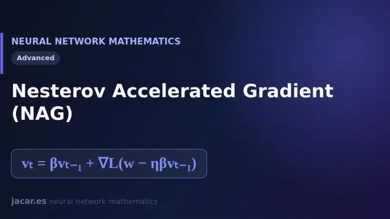
Nesterov accelerated gradient improves classic momentum by evaluating the gradient at a look-ahead point, the one inertia is about to reach, instead of the current point. That anticipation step corrects the trajectory before overshooting and reaches O(1/k²) convergence on smooth convex problems, the fastest a first-order method can achieve.
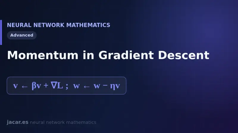
Momentum is an improvement to gradient descent that accumulates a velocity from past gradients instead of looking only at the current one. With a coefficient β around 0.9, that inertia smooths the zigzag of plain SGD, pushes through long narrow valleys and makes training converge noticeably faster than gradient descent alone.
In large neural networks the loss surface almost never traps training in a bad local minimum. The real obstacle is saddle points, far more common in high dimensions. This article explains local versus global minima, why stochastic gradient descent slips past them, and what role convexity plays in the whole picture of optimisation.
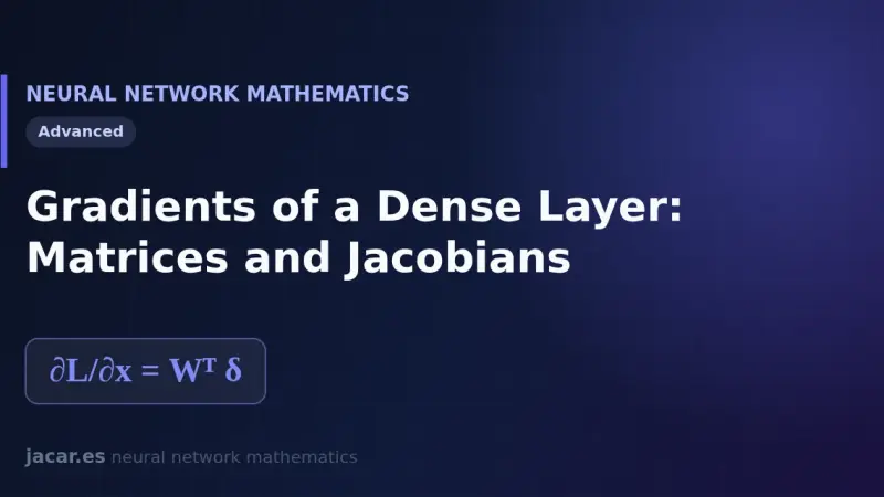
In a dense layer with z equal to Wx plus b, the Jacobian matrix of the output with respect to the input is the weight matrix W itself. From it come the two training rules: the gradient with respect to the weights is delta times x transposed, and the gradient with respect to the input is W transposed times delta.
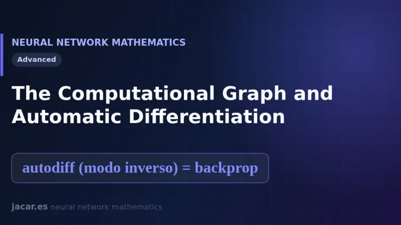
A computational graph represents a function as a network of elementary operations. Automatic differentiation traverses that graph to compute exact derivatives: reverse mode, the basis of backpropagation, obtains the gradient of every weight in a single backward pass. It is the mechanism that makes training networks with billions of parameters possible.
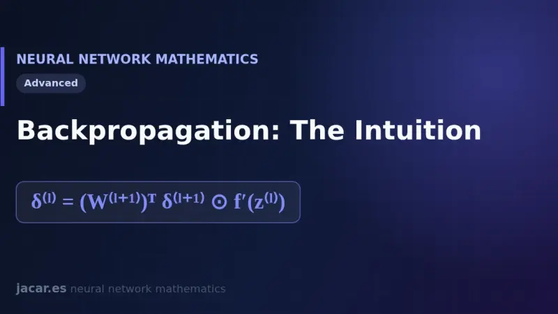
Backpropagation applies the chain rule to share a network's error layer by layer. You first compute the error of the output layer, propagate it backward, and use it to obtain the gradients of every weight and bias in a single pass, summarised in four compact equations you can code directly.
Backpropagation shares out the blame for the error among all the weights of a neural network. It propagates an error signal backwards layer by layer, multiplying by the local derivatives, and so obtains the gradient of every weight in a single pass. That idea, published in 1986, is what makes training deep networks possible.
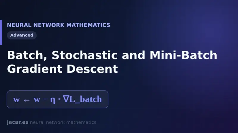
Batch gradient descent uses all the data at each step, the stochastic version uses a single sample and mini-batch picks an intermediate group, usually 32 to 256 examples. This guide compares the three variants, their cost, their noise and why mini-batch has become the standard for training modern networks.
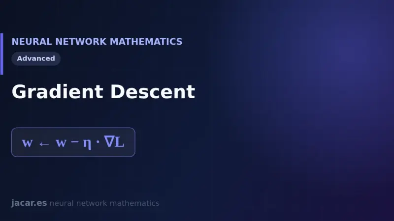
Gradient descent is the algorithm that trains almost every neural network. It computes the slope of the loss function with respect to each weight and takes a small step in the opposite direction, controlled by the learning rate, until it reaches a minimum where the error stops falling and the model has converged.
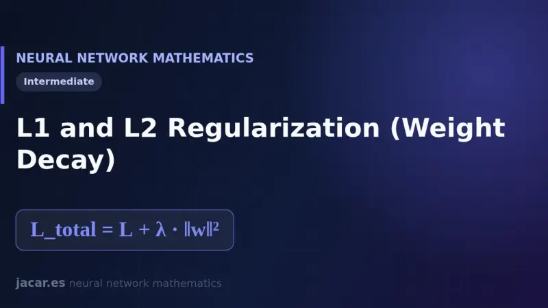
L1 and L2 regularization adds a term to the loss function that penalises large weights. L2, or weight decay, shrinks the weights smoothly towards zero; L1 drives them exactly to zero and yields sparse models. Both curb overfitting and improve the generalisation ability of a neural network on unseen data.
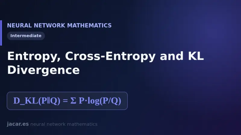
Entropy measures the average uncertainty of a distribution in bits, cross-entropy measures the cost of coding the real data with a wrong model, and KL divergence is the gap between the two. That is why minimising cross-entropy during training is the same as minimising the KL divergence from the labels.
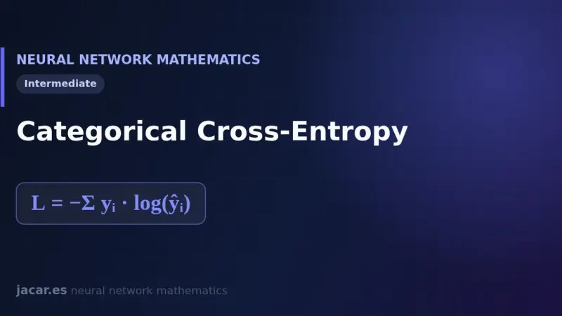
Categorical cross-entropy is the standard loss function for classifying into several mutually exclusive classes. It compares the distribution the network predicts, usually after a softmax, with the true label written in one-hot format, and it penalises heavily any low probability assigned to the correct class.
7 min
We use first- and third-party cookies to analyze site traffic. You can accept them, reject them, or configure your choice.
Learn more about cookies
Cookie preferences
NecessaryEssential for the site to work. Always on.
AnalyticsHelp us understand how the site is used (Google Analytics).