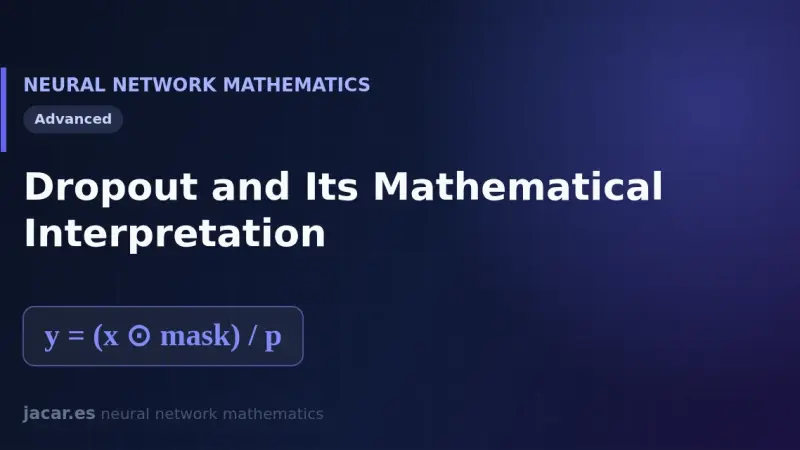
Dropout is a regularization technique that switches neurons off at random during training, with retention probability p, and divides the surviving activations by p to preserve their scale. At inference the full network runs without dropping anything. Mathematically it amounts to averaging a huge ensemble of subnetworks that share weights.
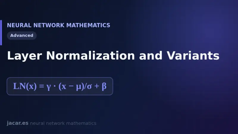
Layer normalization stabilizes training by normalizing each example on its own, using the mean and standard deviation of its own activations. Unlike batch normalization, it does not depend on the batch size, which is why transformers adopted it. RMSNorm is its lighter, most widely used variant today in large language models.
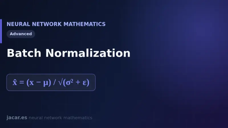
Batch normalization is a technique that normalises each layer's activations using the mean and variance of the mini-batch, then rescales them with two learnable parameters, gamma and beta. Introduced in 2015, it enables higher learning rates, speeds up training and stabilises deep neural networks during optimisation.
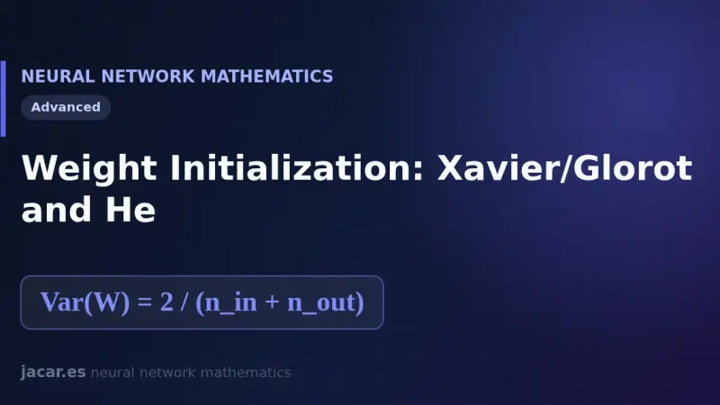
Weight initialization sets the starting scale of the matrix W before training begins. Xavier/Glorot, from 2010, splits the variance between inputs and outputs and suits sigmoid and tanh; He, from 2015, doubles it for ReLU, which zeroes half the activations. A poor choice stalls or breaks learning.
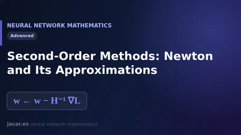
Second-order methods use the Hessian, the matrix of second derivatives of the loss, to orient each step better than the gradient alone. Newton's method updates the weights by subtracting the inverse Hessian times the gradient, but inverting it is far too costly in large networks, so practitioners fall back on quasi-Newton approximations.
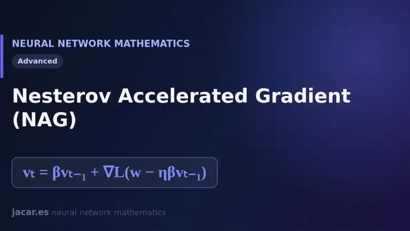
Nesterov accelerated gradient improves classic momentum by evaluating the gradient at a look-ahead point, the one inertia is about to reach, instead of the current point. That anticipation step corrects the trajectory before overshooting and reaches O(1/k²) convergence on smooth convex problems, the fastest a first-order method can achieve.
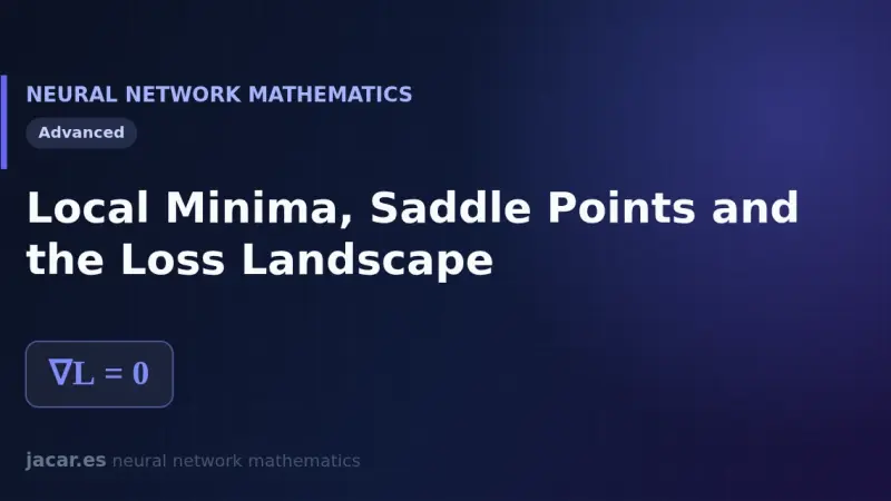
In large neural networks the loss surface almost never traps training in a bad local minimum. The real obstacle is saddle points, far more common in high dimensions. This article explains local versus global minima, why stochastic gradient descent slips past them, and what role convexity plays in the whole picture of optimisation.
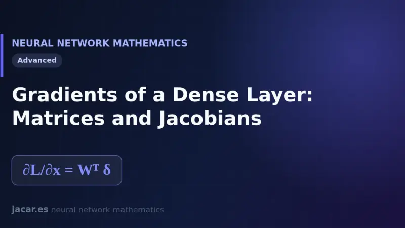
In a dense layer with z equal to Wx plus b, the Jacobian matrix of the output with respect to the input is the weight matrix W itself. From it come the two training rules: the gradient with respect to the weights is delta times x transposed, and the gradient with respect to the input is W transposed times delta.
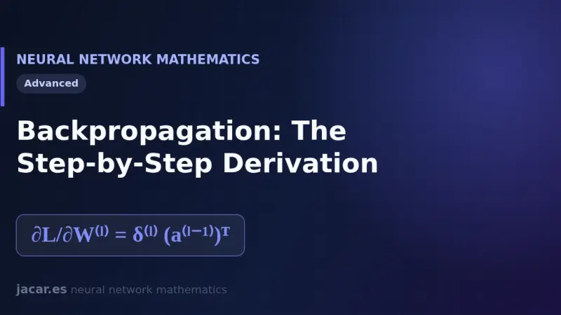
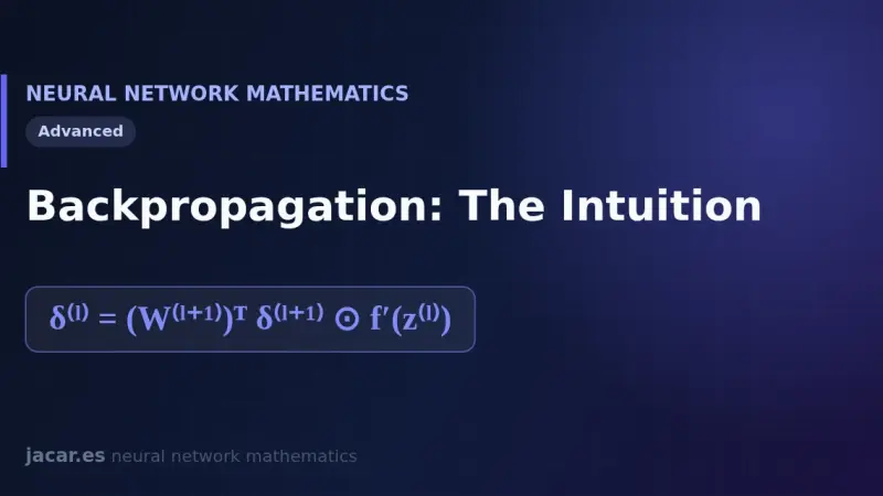
Backpropagation applies the chain rule to share a network's error layer by layer. You first compute the error of the output layer, propagate it backward, and use it to obtain the gradients of every weight and bias in a single pass, summarised in four compact equations you can code directly.
Backpropagation shares out the blame for the error among all the weights of a neural network. It propagates an error signal backwards layer by layer, multiplying by the local derivatives, and so obtains the gradient of every weight in a single pass. That idea, published in 1986, is what makes training deep networks possible.
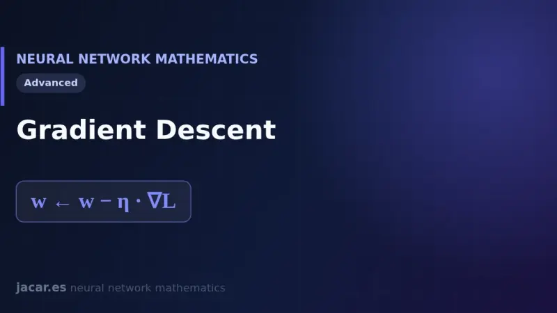
Gradient descent is the algorithm that trains almost every neural network. It computes the slope of the loss function with respect to each weight and takes a small step in the opposite direction, controlled by the learning rate, until it reaches a minimum where the error stops falling and the model has converged.
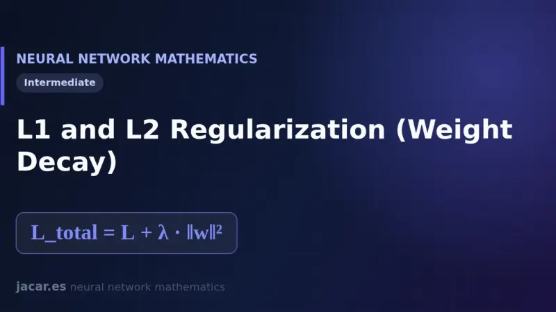
L1 and L2 regularization adds a term to the loss function that penalises large weights. L2, or weight decay, shrinks the weights smoothly towards zero; L1 drives them exactly to zero and yields sparse models. Both curb overfitting and improve the generalisation ability of a neural network on unseen data.
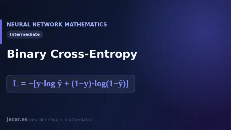
Binary cross-entropy is the standard loss function for two-class classification. It compares the probability returned by the sigmoid with the true label, 0 or 1, and punishes confident mistakes hard. Its formula comes from maximum likelihood, and its derivative combines with the sigmoid into a very simple gradient.
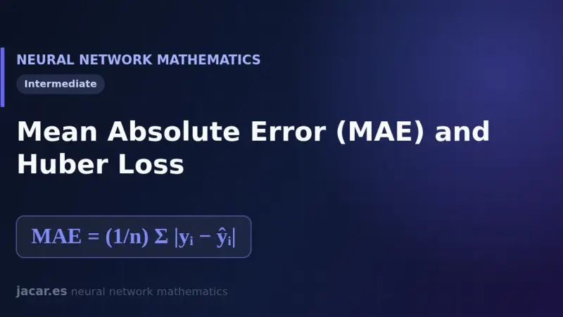
Mean absolute error (MAE) averages the absolute difference between prediction and reality, so a single outlier weighs only its fair share and never blows up the loss. Huber loss combines that robustness with the smoothness of mean squared error through a delta parameter that decides where the behaviour switches over.
A loss function measures how wrong a neural network is on a single example, comparing its prediction with the correct value. The cost function averages that loss across the whole dataset. That single number is exactly what training tries to reduce, step by step, using gradient descent to adjust every weight.
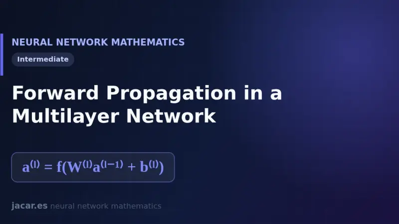
Forward propagation is the process by which a neural network turns its input into a prediction, one layer at a time. Each layer multiplies the input vector by a weight matrix, adds a bias and applies an activation function, so the output of one layer feeds the next until the final result appears at the end.
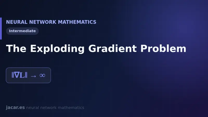
The exploding gradient problem happens when the gradient norm grows without control during backpropagation, especially in deep and recurrent networks with large weights. Training destabilises and the loss turns into NaN. Gradient clipping, together with good initialisation and normalisation, is the standard fix used today.
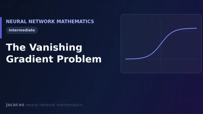
The vanishing gradient problem appears when the error signal shrinks as it backpropagates through many layers. The sigmoid and hyperbolic tangent functions have small derivatives, and their product tends toward zero, so the early layers barely learn. ReLU, careful initialisation and normalisation solve the problem.
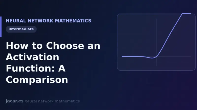
Choosing an activation function is simple with one base rule: use ReLU in the hidden layers, GELU or SiLU in transformers, and reserve the output for softmax in multiclass classification, sigmoid in binary problems and a linear activation in regression. This comparison gathers formulas, ranges and use cases.
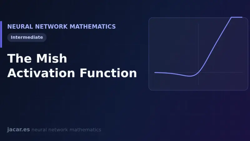
The Mish function is defined as mish(x) = x·tanh(softplus(x)). It is smooth, non-monotonic and self-regularized, properties that let it outperform Swish and ReLU across many tests. The YOLOv4 object detector adopted it in its backbone as the default activation.
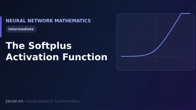
The Softplus function is defined as softplus(x) = ln(1 + eˣ): a smooth, always-positive approximation of ReLU whose derivative is exactly the sigmoid. It is differentiable across its whole domain, avoids ReLU's angular kink and its output never quite reaches zero.
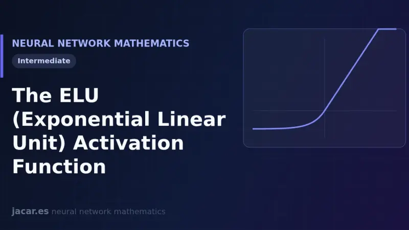
The ELU (Exponential Linear Unit) activation function returns x for positive inputs and α(eˣ−1) for negative ones. By allowing smooth negative values, it pushes the mean of the activations toward zero, speeds up convergence compared with ReLU, and avoids dead neurons thanks to a gradient that never vanishes completely on the negative side.
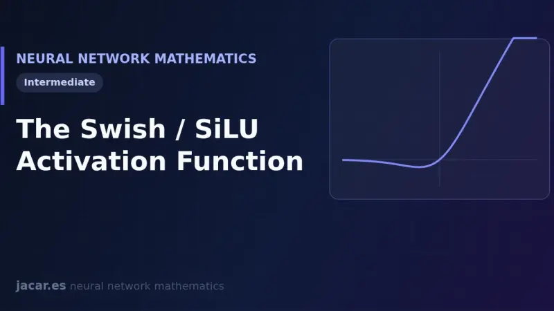
The Swish function, also called SiLU, multiplies the input by its sigmoid: swish(x) = x·σ(x). It is smooth, non-monotonic and self-gating, so it often beats ReLU in deep networks. Models like LLaMA and EfficientNet use it as their default activation.
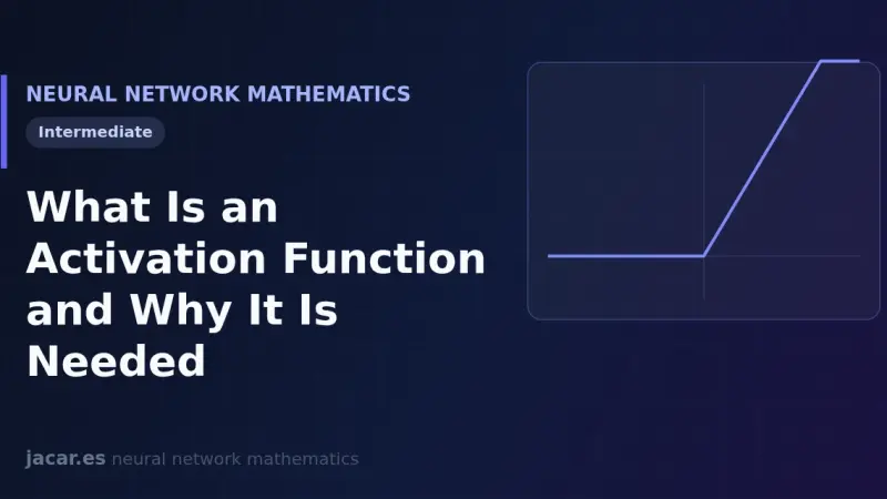
An activation function is the nonlinear operation each neuron applies to its weighted sum z to produce its output a equals f of z. Without it, stacking layers only chains linear transformations and the whole network collapses into a single one. That nonlinearity is what lets a network learn complex patterns.
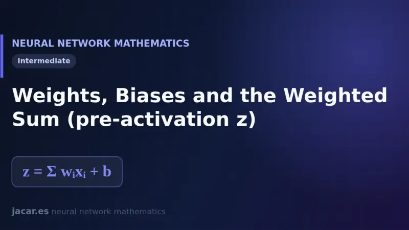
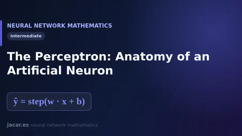
In an artificial neuron, weights measure how important each input is and the bias shifts the result. The neuron multiplies each input by its weight, adds everything up and includes the bias to produce the weighted sum z = Wx + b, the number that then passes through the activation function.
The perceptron is the simplest artificial neuron: it takes several inputs, multiplies them by its weights, adds a bias and applies an activation function that decides between two outputs. Frank Rosenblatt introduced it in 1958, and it remains the basic building block of every modern neural network.
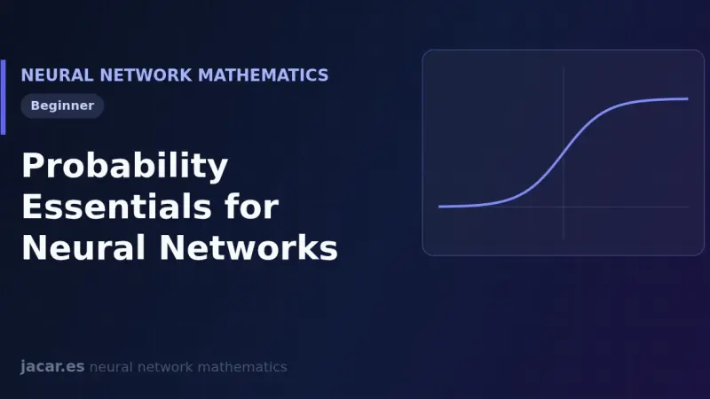
Probability in neural networks rests on three ideas: a distribution assigns weights to possible outcomes, the expected value averages those outcomes, and likelihood measures how well the model fits the data. From those three pieces come the softmax function and the cross-entropy loss that we optimise.
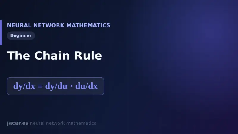
The chain rule computes the derivative of a composite function by multiplying the derivatives of its links: if y depends on u and u depends on x, then dy/dx equals dy/du times du/dx. That layer-by-layer multiplication of derivatives is exactly what backpropagation does to train a neural network.
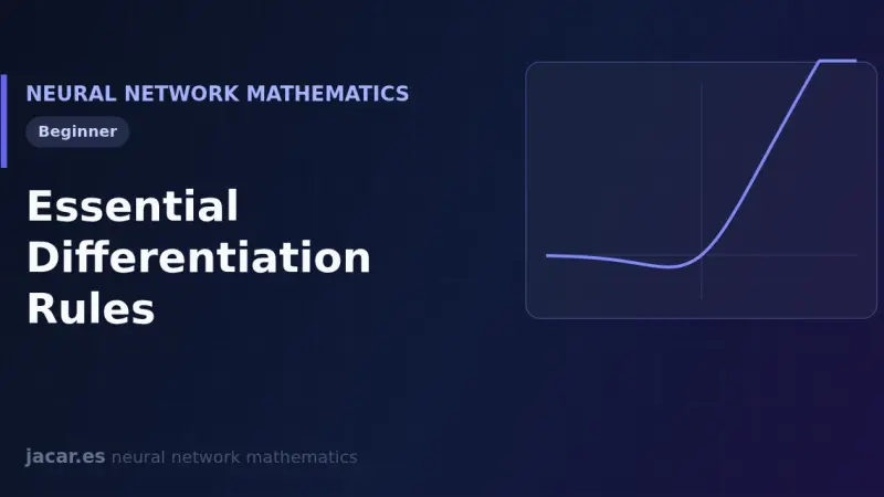
The essential differentiation rules are a handful of formulas that turn any function into its derivative: the power rule, the product and quotient rules, and the rules for the exponential and the logarithm. With them, plus the chain rule, a neural network computes gradients and learns by adjusting its weights.
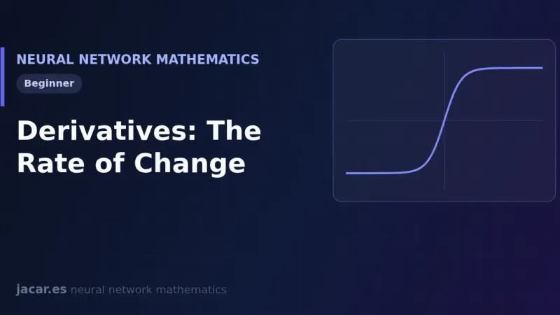
A derivative measures the rate of change of a function: how much its output varies when the input changes a little. In a neural network, that slope tells us in which direction and how strongly to adjust each weight to reduce the error, and it is the foundation of gradient descent and backpropagation.
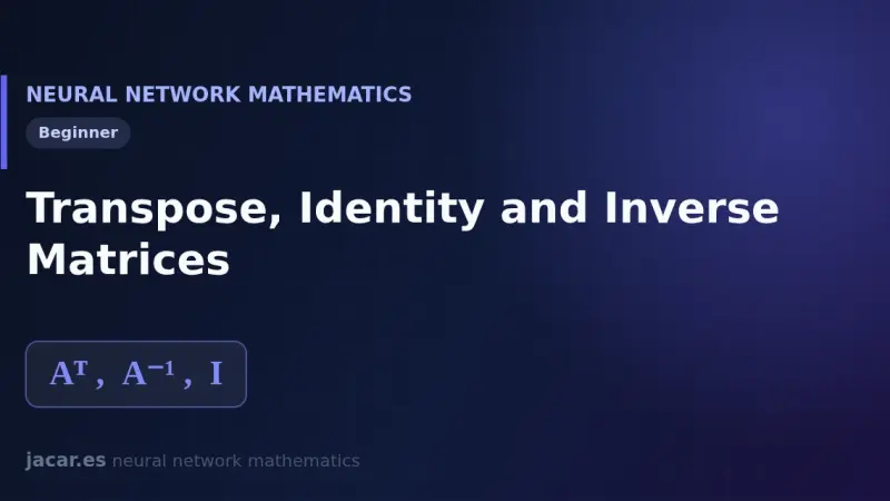
The transpose swaps rows for columns and shows up at every step of backpropagation; the identity matrix acts as the 1 of matrix algebra and leaves any vector unchanged, and the inverse matrix undoes a transformation, though it only exists when the matrix is square and its determinant is not zero. Three operations that hold up the maths of a network.
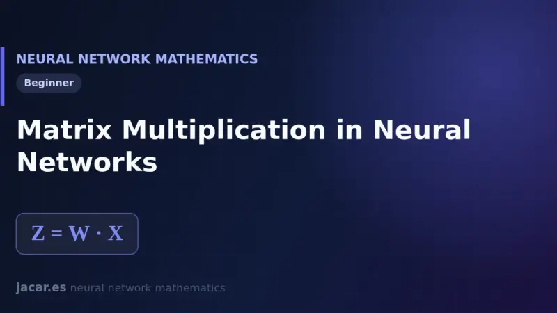
Matrix multiplication is the core operation of a neural network: each layer gathers its weights into a matrix W and computes its output as the product W times X. That single operation, repeated layer after layer, turns the inputs into predictions and explains why graphics cards dominate modern deep learning.
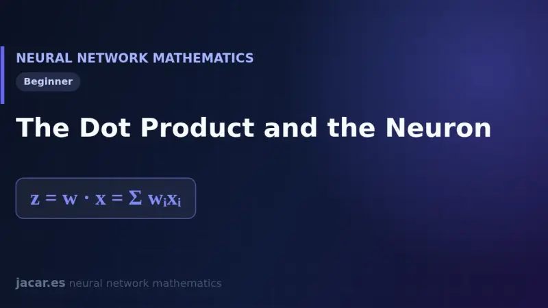
The dot product multiplies each input by its weight and adds the results into a single number. A neuron uses that operation to compute its weighted sum z equals w times x plus the bias b, and that value decides, after the activation, how strongly the neuron fires in response to the data it receives.
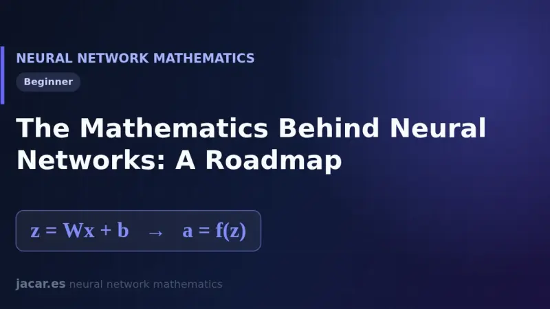
The mathematics of neural networks rests on three blocks: linear algebra represents data and weights as vectors and matrices, calculus with derivatives and the chain rule lets the network learn through gradient descent, and probability shapes the loss functions. This roadmap walks that path from beginning to end so you know what to study and in what order.
6 min2
We use first- and third-party cookies to analyze site traffic. You can accept them, reject them, or configure your choice.
Learn more about cookies
Cookie preferences
NecessaryEssential for the site to work. Always on.
AnalyticsHelp us understand how the site is used (Google Analytics).