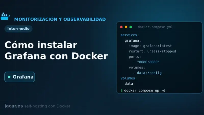
Grafana is the most widely used open-source platform for building dashboards and visualising metrics, and with Docker you bring it up with a single docker-compose.yml. It listens on port 3000, stores its data in /var/lib/grafana and connects to Prometheus, Loki or InfluxDB as data sources. Here you install it, provision it and publish it with Traefik.
Node Exporter and cAdvisor are the two exporters that feed Prometheus: the first collects host metrics (CPU, RAM, disk and network) on port 9100, and the second collects per-container metrics on port 8080. This guide brings both up with a single docker-compose.yml, connects them to Prometheus and explains which metrics to watch.
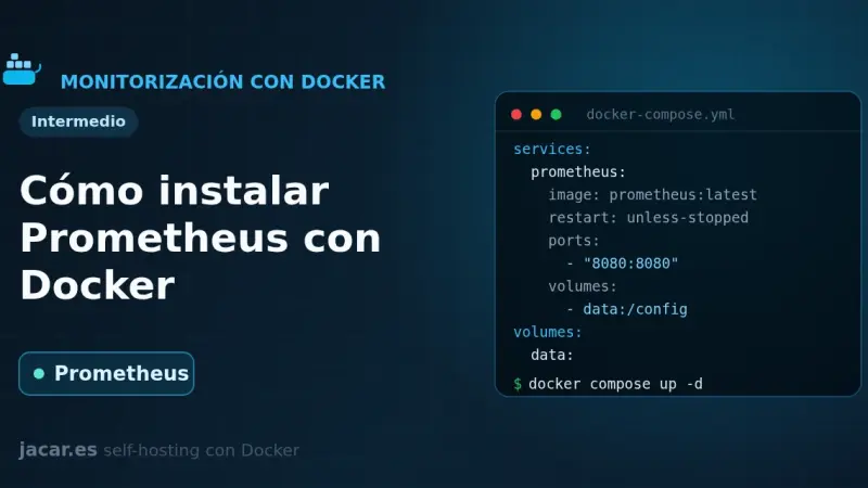
Prometheus is the most widely adopted open-source monitoring and alerting system for self-hosted infrastructure, and with Docker you bring it up with a single docker-compose.yml and a prometheus.yml. It collects metrics using a pull model, stores them in its time-series database and exposes them on port 9090, ready to query with PromQL and visualise in Grafana.
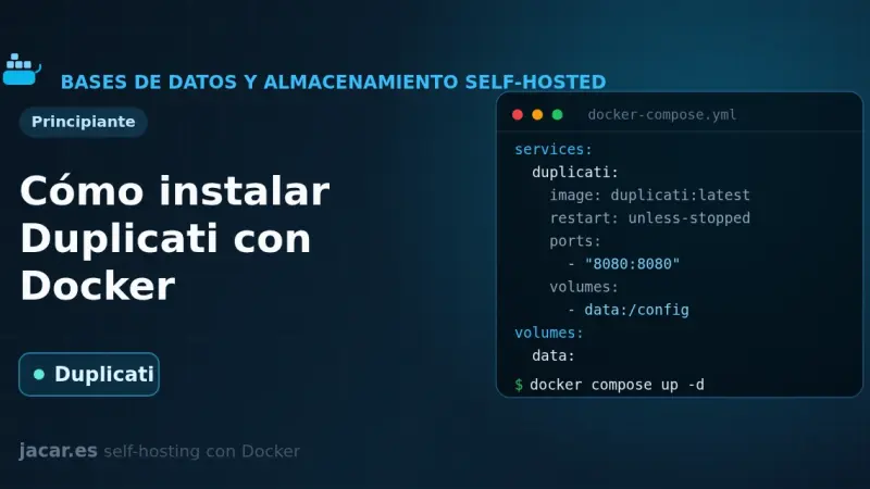
Duplicati is a free backup tool that encrypts your data with AES-256 before sending it and only uploads the blocks that have changed. With Docker you bring it up from a single docker-compose.yml, mount your folders read-only and schedule encrypted backups to S3, MinIO, B2 or SFTP. This guide covers installation, encryption, retention and restore.
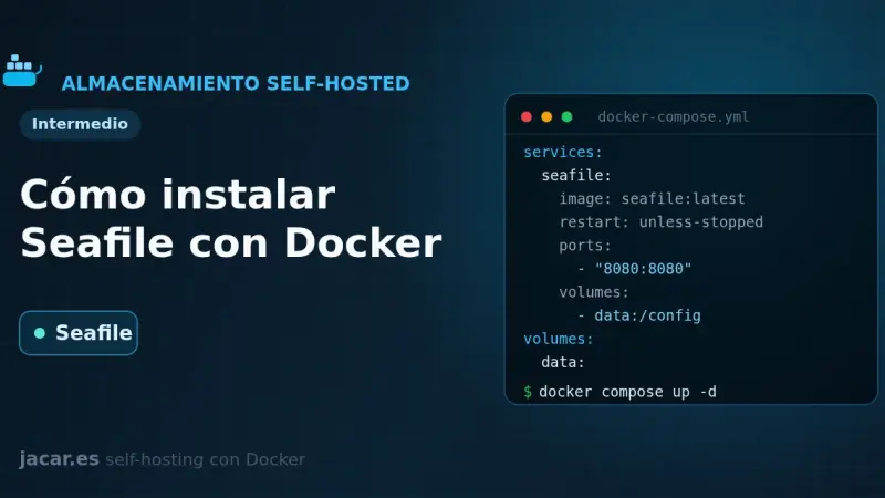
Seafile is an open-source file sync and storage platform that keeps data in blocks, Git style, which makes it very fast when you handle lots of files. With Docker it comes up in four containers (server, a MariaDB database, a Redis cache and a Caddy proxy) from a single docker-compose.yml file.
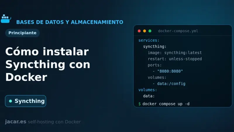
Syncthing is a free peer-to-peer file synchronisation tool: it keeps folders identical across your devices without going through the cloud and with all traffic encrypted. With Docker you bring it up from a single docker-compose.yml using host networking, PUID/PGID for permissions and a persistent volume. This guide covers the installation, device pairing and the ports you need.
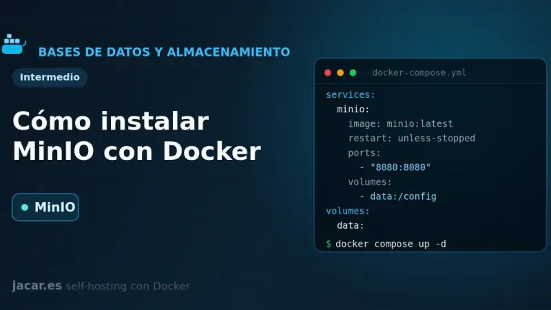
MinIO is an object storage server compatible with the Amazon S3 API that you can self-host with Docker. With a single docker-compose.yml you bring up the API on port 9000 and the console on 9001, create buckets and access keys with the mc client, and use it as an S3 backend for backups, attachments and photos.
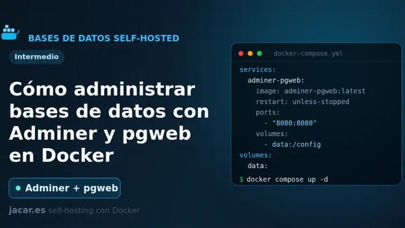
Adminer and pgweb are two web-based database managers that run in Docker with a single container each. Adminer is one PHP file that handles MySQL, PostgreSQL and six other engines; pgweb is a Go explorer dedicated to PostgreSQL. This guide brings a ready-to-copy docker-compose.yml and explains how to secure them properly.
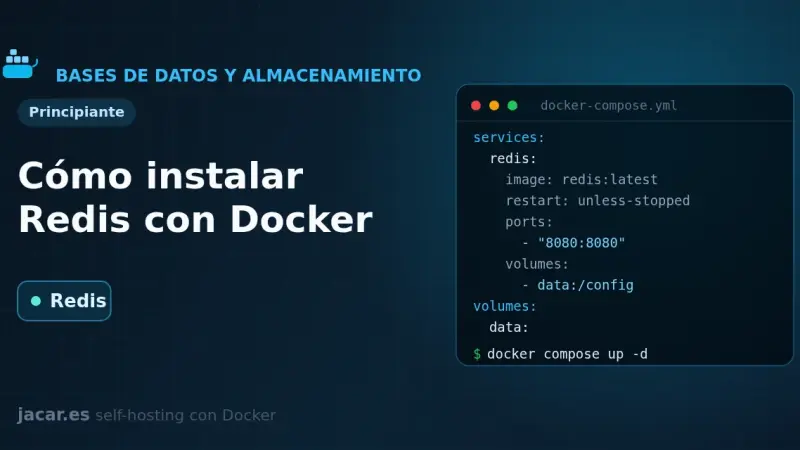
Redis is an in-memory key-value data store used as a cache, a job queue and a session manager. With Docker you bring it up from a single docker-compose.yml file, with persistence on a volume, a mandatory password and a healthcheck. This guide covers the installation, how to secure it and how it differs from Valkey.
MariaDB is an open-source relational database, a fork of MySQL and compatible with it, that in Docker runs as a single container with a persistent volume. With this docker-compose.yml you set the root password, the database and the initial user through environment variables, and you keep your data even if you recreate the container.
PostgreSQL is the most advanced open-source relational database, and in Docker you bring it up with a single docker-compose.yml file. You define a persistent volume, the superuser password and a pg_isready healthcheck, and within seconds you have a server on port 5432 ready for other containers to connect to it by the service name.
Firefly III is an open-source personal finance manager you self-host with Docker. With one docker-compose.yml file you bring up the application, a MariaDB database and the data importer, which connects to more than 6,000 banks through GoCardless. You generate the 32-character APP_KEY and keep control of all your money on your own server.
Stirling-PDF is a web-based Swiss Army knife for PDFs that you self-host with Docker in a single container. With one docker-compose.yml file you bring up more than fifty tools to merge, split, compress, convert, sign and OCR your documents, all processed on your own server and without sending anything to the cloud.
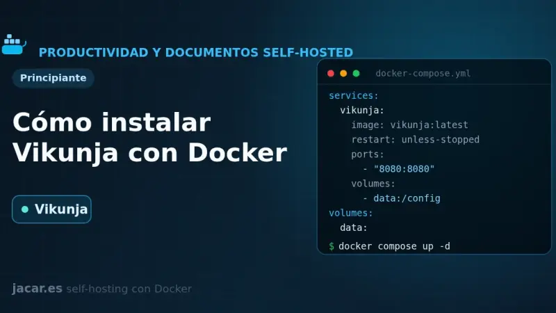
Vikunja is an open-source task manager that you self-host with Docker in a single image. With one docker-compose.yml file you bring up the application alongside a PostgreSQL database and organize your projects in list, kanban board, Gantt and table views, with all your data stored on your own server.
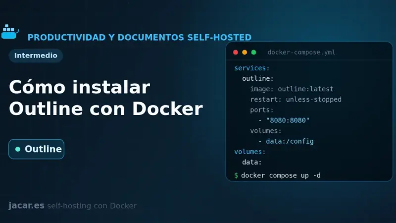
Outline is a source-available team wiki and knowledge base that in Docker needs three pieces: PostgreSQL, Redis and a login provider, because it ships with no local username and password. With one docker-compose.yml file you bring up the service, connect it to Authentik over OIDC and store attachments in MinIO.
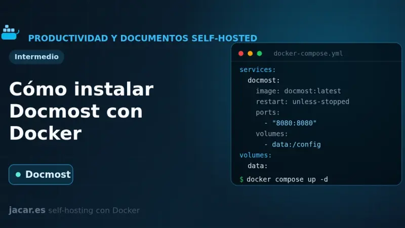
Docmost is an open-source wiki and knowledge base, a self-hosted alternative to Confluence and Notion. On Docker it runs as three containers: the application, a PostgreSQL database and a Redis cache. A single docker-compose.yml file gives you workspaces, real-time collaborative editing and full control over your documents.
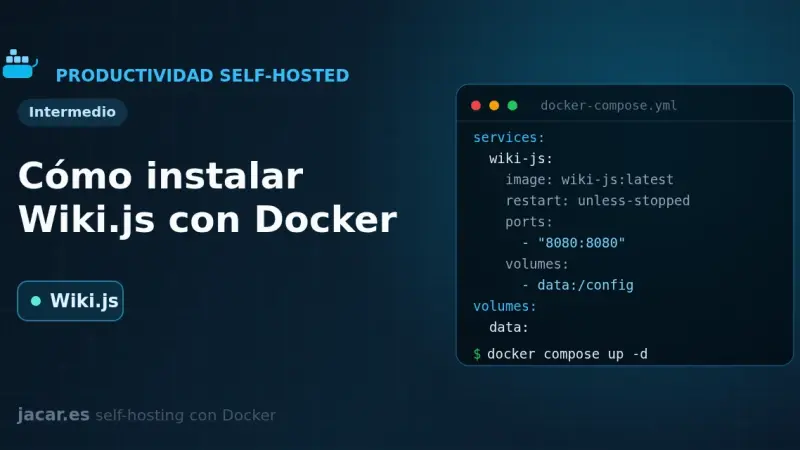
Wiki.js is an open-source wiki engine written in Node.js that, in Docker, runs as two containers: the application and a PostgreSQL database. With a single docker-compose.yml file you get your own wiki with a Markdown editor, version control and more than forty authentication methods, and your pages stored in a volume that you control.
BookStack is an open-source documentation wiki platform, written in PHP with Laravel, that organises content into shelves, books, chapters and pages. With Docker it installs in minutes using the LinuxServer image alongside a MariaDB database, and you only need to set APP_URL and APP_KEY in a single docker-compose.yml file.
Paperless-ngx is an open-source document manager that digitises and archives your papers with full-text search. In Docker it runs as five containers (application, PostgreSQL database, Valkey queue, Gotenberg and Tika) through a single docker-compose.yml, and it performs OCR and automatic tagging on every document you drop into its consume folder.
Nextcloud is an open-source private cloud platform that, in Docker, runs as three containers: the application, a MariaDB database and a Redis cache. With a single docker-compose.yml file you get your own self-hosted Drive, calendar and contacts in minutes, with your data stored in a volume that you control.
Watchtower is a container that watches your Docker registries, detects when a newer image is available, pulls it and recreates your container with the same options. You configure it with a small docker-compose.yml, it polls every 24 hours by default, and you can restrict it with labels or keep it in notify-only mode.
A private Docker registry is your own image store: the official registry image listens on port 5000, keeps layers in a volume and, with htpasswd authentication in bcrypt format and HTTPS behind a reverse proxy, lets you push and pull images without depending on Docker Hub or its pull-rate limits.
By default Docker limits neither the CPU nor the RAM of a container: a single one can exhaust the whole server. In Compose you bound them with deploy.resources.limits (cpus, memory) or the mem_limit and cpus shortcuts, and you control logs with the local driver, which rotates at 20 MB and 5 files by default.
Docker Compose profiles tag services so they only start when you enable their profile with --profile or COMPOSE_PROFILES. Services without a profile always run; tagged ones stay idle until you ask for them. That lets a single file hold the core stack, debugging tools and optional extras without duplicate compose files.
A healthcheck is a command Docker runs periodically inside the container to decide whether the service is healthy; its state moves from starting to healthy or unhealthy. Combined with a restart policy (no, always, on-failure or unless-stopped) and with depends_on and the service_healthy condition, it stops an application from starting before its database.
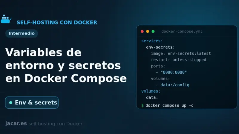
Docker Compose gives you three ways to pass configuration into a container: the environment key, the env_file attribute and the .env file for interpolation. For sensitive data, do not use environment variables; Docker Compose secrets are mounted as read-only files under /run/secrets/, away from logs and the process environment.
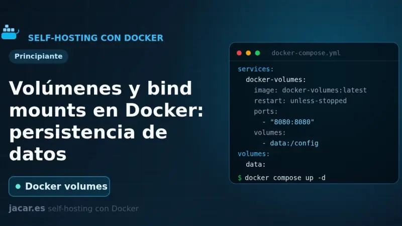
A container loses its data the moment you delete it, unless you store that data outside. Docker gives you two ways: named volumes, which it manages itself under /var/lib/docker/volumes, and bind mounts, which link a host folder. Here you will see when to use each, how to mount them in Compose and how to back them up.
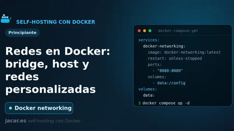
Docker ships six network drivers: bridge, host, none, overlay, macvlan and ipvlan. The default bridge network connects containers by IP but without name resolution. A user-defined bridge adds an internal DNS server so services find each other by name, and it is the recommended choice for almost any deployment.
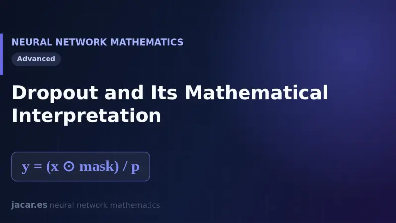
Dropout is a regularization technique that switches neurons off at random during training, with retention probability p, and divides the surviving activations by p to preserve their scale. At inference the full network runs without dropping anything. Mathematically it amounts to averaging a huge ensemble of subnetworks that share weights.
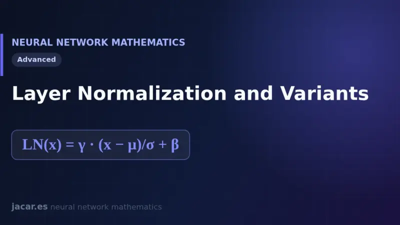
Layer normalization stabilizes training by normalizing each example on its own, using the mean and standard deviation of its own activations. Unlike batch normalization, it does not depend on the batch size, which is why transformers adopted it. RMSNorm is its lighter, most widely used variant today in large language models.
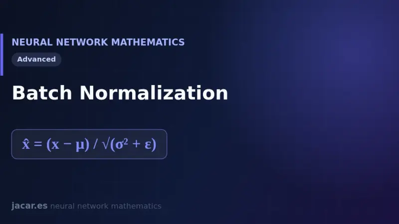
Batch normalization is a technique that normalises each layer's activations using the mean and variance of the mini-batch, then rescales them with two learnable parameters, gamma and beta. Introduced in 2015, it enables higher learning rates, speeds up training and stabilises deep neural networks during optimisation.
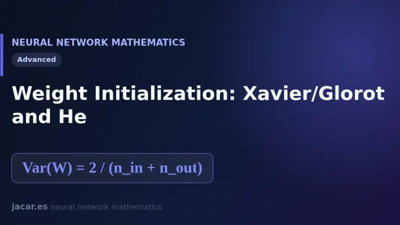
Weight initialization sets the starting scale of the matrix W before training begins. Xavier/Glorot, from 2010, splits the variance between inputs and outputs and suits sigmoid and tanh; He, from 2015, doubles it for ReLU, which zeroes half the activations. A poor choice stalls or breaks learning.
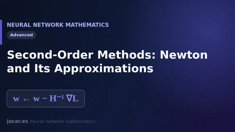
Second-order methods use the Hessian, the matrix of second derivatives of the loss, to orient each step better than the gradient alone. Newton's method updates the weights by subtracting the inverse Hessian times the gradient, but inverting it is far too costly in large networks, so practitioners fall back on quasi-Newton approximations.
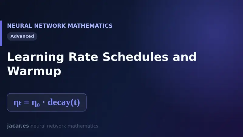
A learning rate schedule changes the value of η over the course of training instead of keeping it fixed. It starts with a warmup that raises η from near zero, holds a peak and then lowers it with step, exponential or cosine decay so the network converges faster and with far less oscillation.
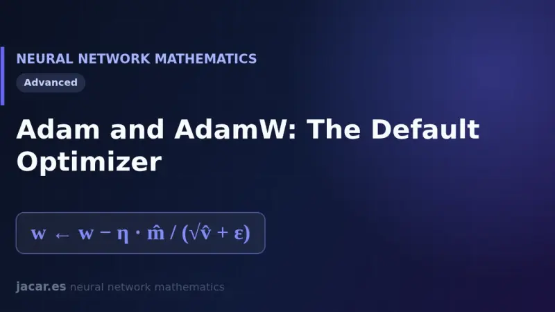
Adam combines a first-order moment (a moving average of the gradient) and a second-order moment (an average of its squares) to give each parameter its own learning rate. With bias correction and the defaults β1=0.9, β2=0.999 and ε=1e-8, it converges fast with almost no tuning.
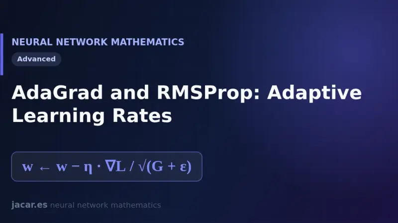
AdaGrad and RMSProp are optimisers that give every weight its own learning rate. AdaGrad accumulates the square of all past gradients and divides the step by its root, which slowly fades it out. RMSProp fixes this with a moving average that forgets the past using a decay factor of about 0.9.
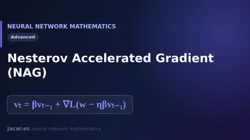
Nesterov accelerated gradient improves classic momentum by evaluating the gradient at a look-ahead point, the one inertia is about to reach, instead of the current point. That anticipation step corrects the trajectory before overshooting and reaches O(1/k²) convergence on smooth convex problems, the fastest a first-order method can achieve.
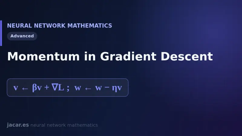
Momentum is an improvement to gradient descent that accumulates a velocity from past gradients instead of looking only at the current one. With a coefficient β around 0.9, that inertia smooths the zigzag of plain SGD, pushes through long narrow valleys and makes training converge noticeably faster than gradient descent alone.
In large neural networks the loss surface almost never traps training in a bad local minimum. The real obstacle is saddle points, far more common in high dimensions. This article explains local versus global minima, why stochastic gradient descent slips past them, and what role convexity plays in the whole picture of optimisation.
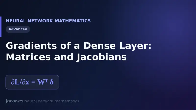
In a dense layer with z equal to Wx plus b, the Jacobian matrix of the output with respect to the input is the weight matrix W itself. From it come the two training rules: the gradient with respect to the weights is delta times x transposed, and the gradient with respect to the input is W transposed times delta.
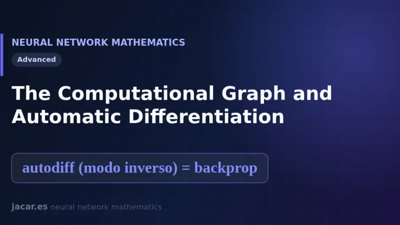
A computational graph represents a function as a network of elementary operations. Automatic differentiation traverses that graph to compute exact derivatives: reverse mode, the basis of backpropagation, obtains the gradient of every weight in a single backward pass. It is the mechanism that makes training networks with billions of parameters possible.
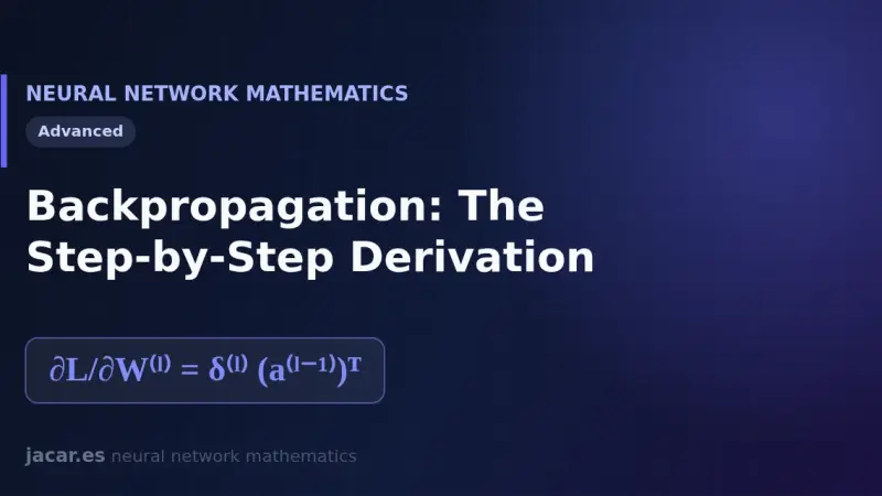
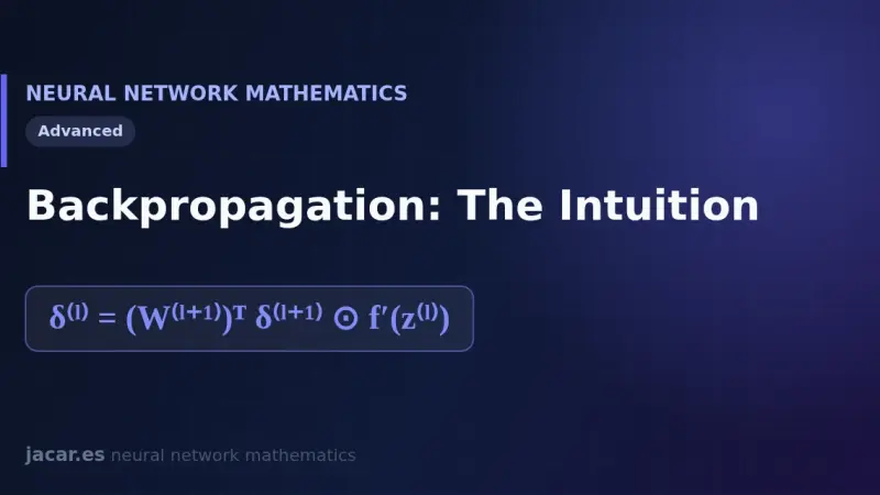
Backpropagation applies the chain rule to share a network's error layer by layer. You first compute the error of the output layer, propagate it backward, and use it to obtain the gradients of every weight and bias in a single pass, summarised in four compact equations you can code directly.
Backpropagation shares out the blame for the error among all the weights of a neural network. It propagates an error signal backwards layer by layer, multiplying by the local derivatives, and so obtains the gradient of every weight in a single pass. That idea, published in 1986, is what makes training deep networks possible.
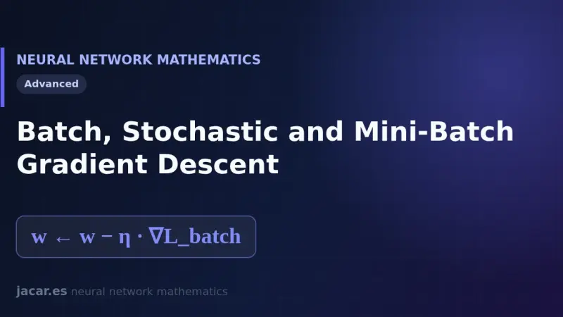
Batch gradient descent uses all the data at each step, the stochastic version uses a single sample and mini-batch picks an intermediate group, usually 32 to 256 examples. This guide compares the three variants, their cost, their noise and why mini-batch has become the standard for training modern networks.
The learning rate is the hyperparameter that sets the size of each step when adjusting the weights during training. Too high a value makes the loss diverge; too low a value makes learning painfully slow. Typical values range from 0.001 with Adam to 0.1 with classic gradient descent.
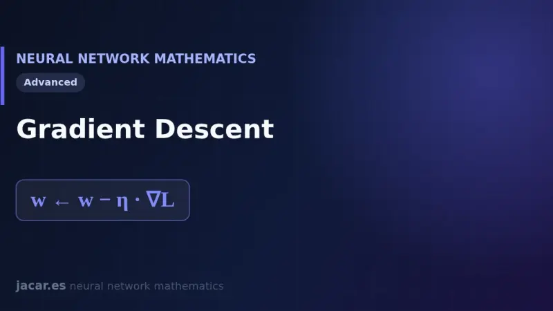
Gradient descent is the algorithm that trains almost every neural network. It computes the slope of the loss function with respect to each weight and takes a small step in the opposite direction, controlled by the learning rate, until it reaches a minimum where the error stops falling and the model has converged.
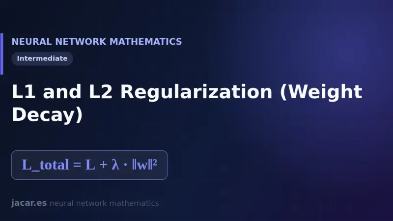
L1 and L2 regularization adds a term to the loss function that penalises large weights. L2, or weight decay, shrinks the weights smoothly towards zero; L1 drives them exactly to zero and yields sparse models. Both curb overfitting and improve the generalisation ability of a neural network on unseen data.
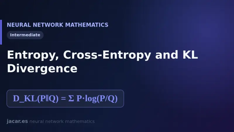
Entropy measures the average uncertainty of a distribution in bits, cross-entropy measures the cost of coding the real data with a wrong model, and KL divergence is the gap between the two. That is why minimising cross-entropy during training is the same as minimising the KL divergence from the labels.
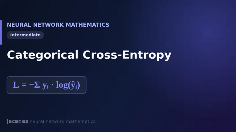
Categorical cross-entropy is the standard loss function for classifying into several mutually exclusive classes. It compares the distribution the network predicts, usually after a softmax, with the true label written in one-hot format, and it penalises heavily any low probability assigned to the correct class.
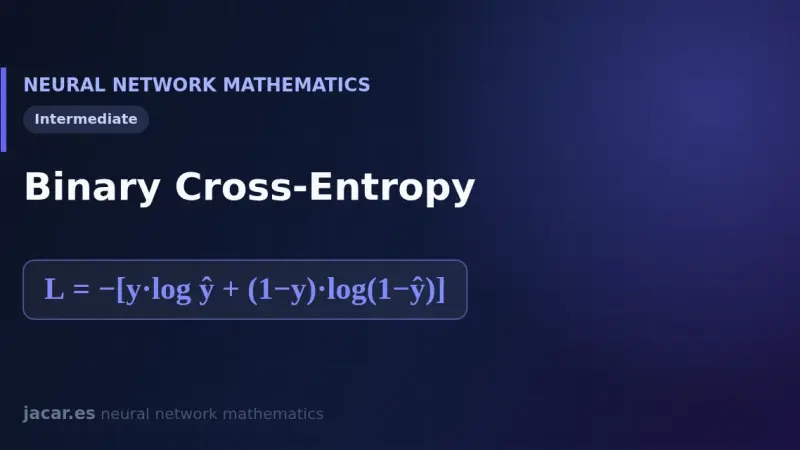
Binary cross-entropy is the standard loss function for two-class classification. It compares the probability returned by the sigmoid with the true label, 0 or 1, and punishes confident mistakes hard. Its formula comes from maximum likelihood, and its derivative combines with the sigmoid into a very simple gradient.
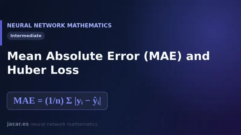
Mean absolute error (MAE) averages the absolute difference between prediction and reality, so a single outlier weighs only its fair share and never blows up the loss. Huber loss combines that robustness with the smoothness of mean squared error through a delta parameter that decides where the behaviour switches over.
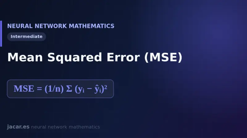
Mean squared error (MSE) is the most common loss function in regression: it averages the square of the gap between each true value and its prediction. Squaring punishes big mistakes hard, keeps the function differentiable and gives gradient descent a clear, smooth target to minimise while training a model.
A loss function measures how wrong a neural network is on a single example, comparing its prediction with the correct value. The cost function averages that loss across the whole dataset. That single number is exactly what training tries to reduce, step by step, using gradient descent to adjust every weight.
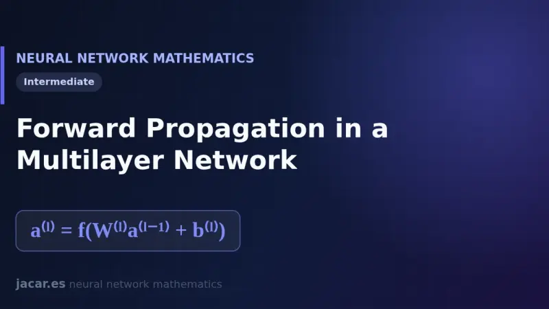
Forward propagation is the process by which a neural network turns its input into a prediction, one layer at a time. Each layer multiplies the input vector by a weight matrix, adds a bias and applies an activation function, so the output of one layer feeds the next until the final result appears at the end.
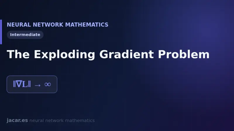
The exploding gradient problem happens when the gradient norm grows without control during backpropagation, especially in deep and recurrent networks with large weights. Training destabilises and the loss turns into NaN. Gradient clipping, together with good initialisation and normalisation, is the standard fix used today.
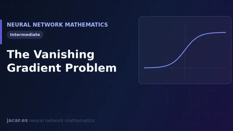
The vanishing gradient problem appears when the error signal shrinks as it backpropagates through many layers. The sigmoid and hyperbolic tangent functions have small derivatives, and their product tends toward zero, so the early layers barely learn. ReLU, careful initialisation and normalisation solve the problem.
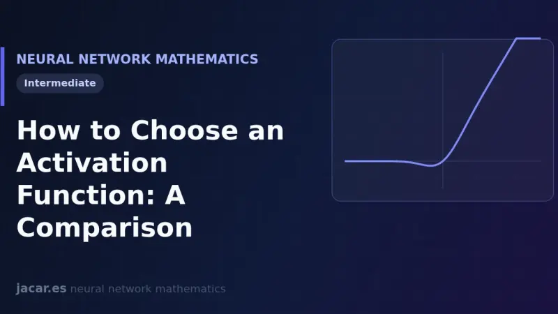
Choosing an activation function is simple with one base rule: use ReLU in the hidden layers, GELU or SiLU in transformers, and reserve the output for softmax in multiclass classification, sigmoid in binary problems and a linear activation in regression. This comparison gathers formulas, ranges and use cases.
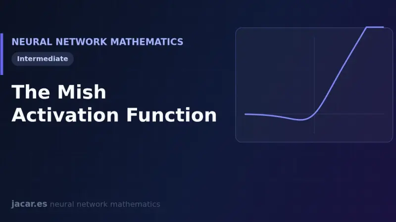
The Mish function is defined as mish(x) = x·tanh(softplus(x)). It is smooth, non-monotonic and self-regularized, properties that let it outperform Swish and ReLU across many tests. The YOLOv4 object detector adopted it in its backbone as the default activation.
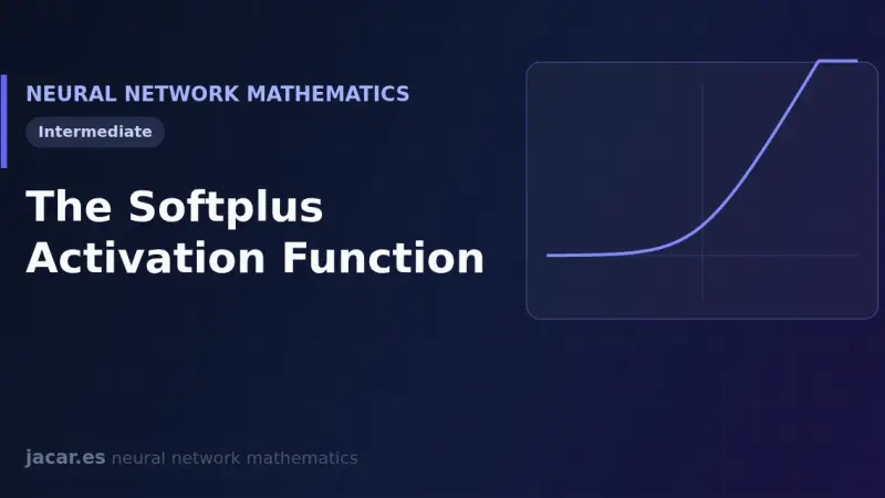
The Softplus function is defined as softplus(x) = ln(1 + eˣ): a smooth, always-positive approximation of ReLU whose derivative is exactly the sigmoid. It is differentiable across its whole domain, avoids ReLU's angular kink and its output never quite reaches zero.
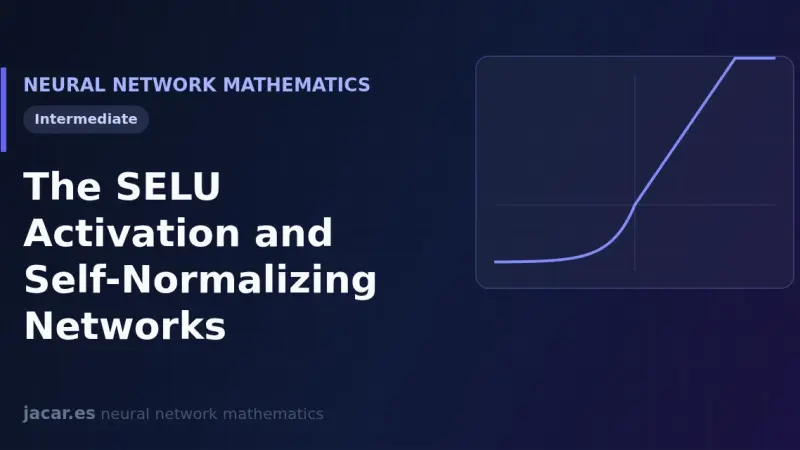
The SELU (Scaled Exponential Linear Unit) function is defined as SELU(x) equal to lambda times ELU(x), with lambda near 1.0507 and alpha near 1.6733. Those two constants make activations converge on their own towards zero mean and unit variance layer after layer, building deep networks that normalize themselves without batch normalization.
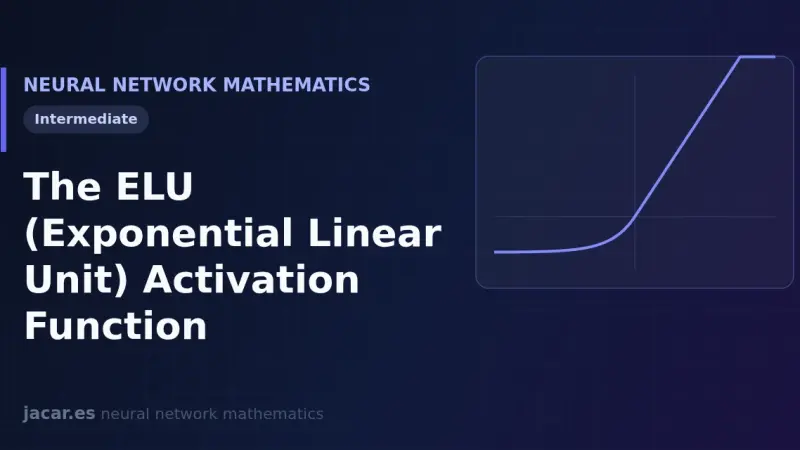
The ELU (Exponential Linear Unit) activation function returns x for positive inputs and α(eˣ−1) for negative ones. By allowing smooth negative values, it pushes the mean of the activations toward zero, speeds up convergence compared with ReLU, and avoids dead neurons thanks to a gradient that never vanishes completely on the negative side.
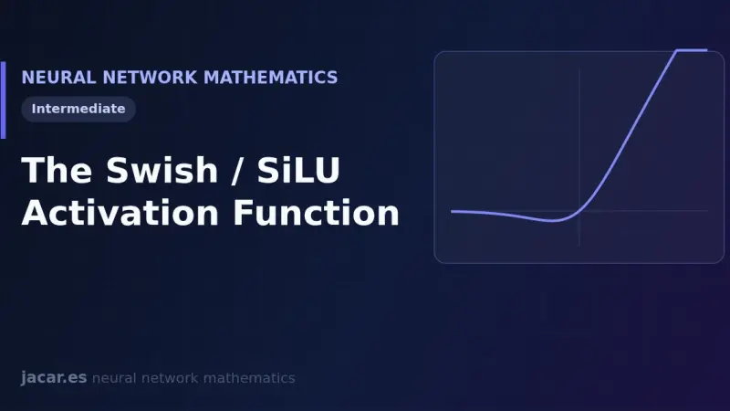
The Swish function, also called SiLU, multiplies the input by its sigmoid: swish(x) = x·σ(x). It is smooth, non-monotonic and self-gating, so it often beats ReLU in deep networks. Models like LLaMA and EfficientNet use it as their default activation.
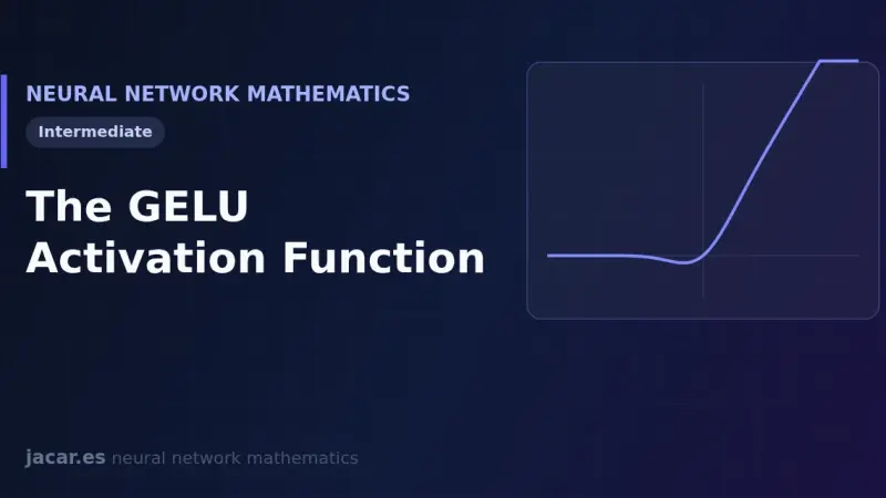
The GELU (Gaussian Error Linear Unit) function multiplies each input by the probability that a standard normal falls below that input. The result is a smooth curve with a continuous derivative that weights inputs by their magnitude, and it has become the default activation inside BERT and GPT.
An activation function is the nonlinear operation each neuron applies to its weighted sum z to produce its output a equals f of z. Without it, stacking layers only chains linear transformations and the whole network collapses into a single one. That nonlinearity is what lets a network learn complex patterns.
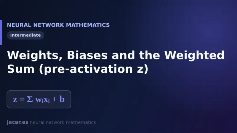
In an artificial neuron, weights measure how important each input is and the bias shifts the result. The neuron multiplies each input by its weight, adds everything up and includes the bias to produce the weighted sum z = Wx + b, the number that then passes through the activation function.
The perceptron is the simplest artificial neuron: it takes several inputs, multiplies them by its weights, adds a bias and applies an activation function that decides between two outputs. Frank Rosenblatt introduced it in 1958, and it remains the basic building block of every modern neural network.
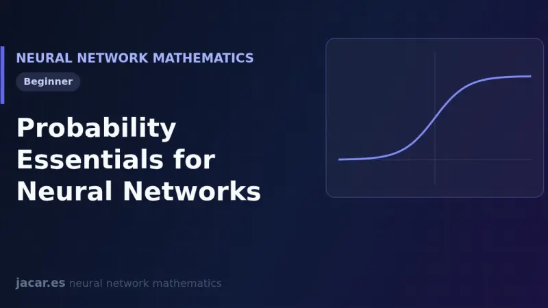
Probability in neural networks rests on three ideas: a distribution assigns weights to possible outcomes, the expected value averages those outcomes, and likelihood measures how well the model fits the data. From those three pieces come the softmax function and the cross-entropy loss that we optimise.
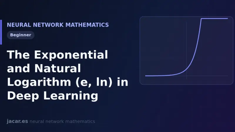
The exponential function eˣ and its inverse, the natural logarithm ln(x), appear again and again in deep learning. The exponential builds the sigmoid and softmax that turn numbers into probabilities, while the natural logarithm defines cross-entropy, the loss used to train almost every classifier in practice today.
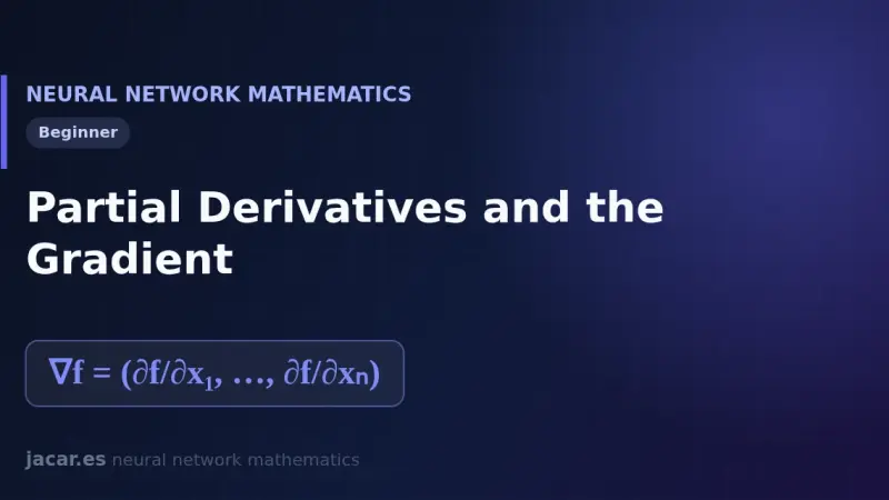
A partial derivative measures how a function changes when you move just one of its variables and hold the rest fixed. The gradient gathers all those partial derivatives into a vector that points toward the steepest ascent; in a neural network, moving the opposite way lowers the error and drives the training.
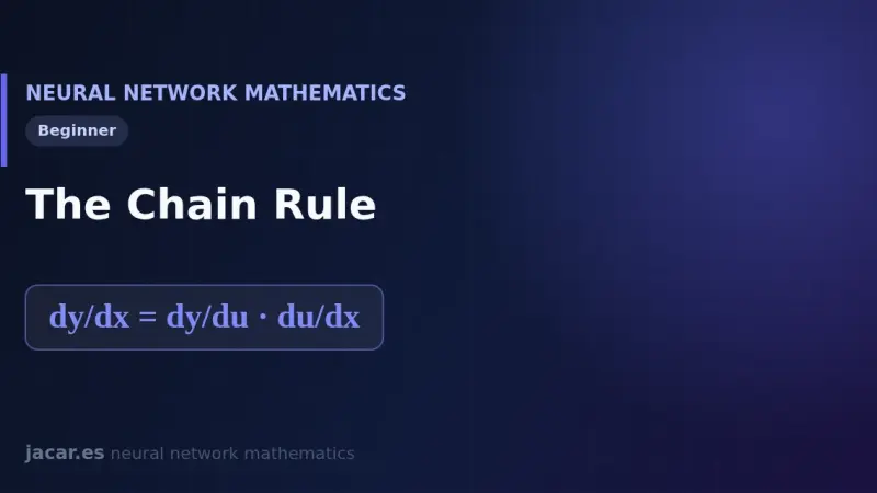
The chain rule computes the derivative of a composite function by multiplying the derivatives of its links: if y depends on u and u depends on x, then dy/dx equals dy/du times du/dx. That layer-by-layer multiplication of derivatives is exactly what backpropagation does to train a neural network.
The essential differentiation rules are a handful of formulas that turn any function into its derivative: the power rule, the product and quotient rules, and the rules for the exponential and the logarithm. With them, plus the chain rule, a neural network computes gradients and learns by adjusting its weights.
A derivative measures the rate of change of a function: how much its output varies when the input changes a little. In a neural network, that slope tells us in which direction and how strongly to adjust each weight to reduce the error, and it is the foundation of gradient descent and backpropagation.
7 min
We use first- and third-party cookies to analyze site traffic. You can accept them, reject them, or configure your choice.
Learn more about cookies
Cookie preferences
NecessaryEssential for the site to work. Always on.
AnalyticsHelp us understand how the site is used (Google Analytics).